Chapter 8 The Binomial Distribution

Figure 8.1: A Statypus Flipping Their Lucky Coin

A platypus will glow under UV or “black” light. It has biofluorescence which is not unique to the platypus, but it is a shining example of what makes the platypus so cool!⁶⁹

The Binomial Distribution arises when someone investigates the number of times someone “succeeds” in a sequence of repeated independent events. For example, if someone flips a fair coin 50 times, we can model how often we expect to see heads. We expect that we would see 25 heads, but there is only around an 11% chance that this will be the case. However, if we allow a little wiggle room, we get that there is an almost 68% chance that there will be between 22 and 28 heads inclusively and an over 88% chance that the number of heads is between 20 and 30 inclusively. If the coin returned 48 heads, we may start to wonder if the coin is “fair” or not. This is because a “fair” coin should only give a result this extreme (or more extreme) one out of every 880 billion sequences of 50 flips.

New R Functions Used

All functions listed below have a help file built into RStudio. Most of these functions have options which are not fully covered or not mentioned in this chapter. To access more information about other functionality and uses for these functions, use the ? command. E.g. To see the help file for qnorm, you can run ?qbinom or ?qbinom() in either an R Script or in your Console.

• dninom(): Probability Density Function for the binomial distribution.

• pbinom(): Cumulative Distribution Function for the binomial distribution.

• qbinom(): Quantile function for the binomial distribution.

• rbinom(): Random number generation for the binomial distribution.

8.1 The Binomial Distribution

The Binomial Distribution will be our archetype of a discrete random variable. It along with a Normal random variable will be our main tools for understanding discrete and continuous random phenomena respectively.

A binomial or Bernoulli⁷⁰ trial is a random experiment which can take one of two values thought of as “Success” and “Failure.” For example, flipping a coin results can be viewed as a Bernoulli trial if we choose if we choose which of “Heads” or “Tails” to consider as a “Success.” Other examples would be shooting free throws on a basketball court, observing a defective product off an assembly line, asking a random person if they will vote “Yes” for a particular referendum, or seeing if the sum of two dice is seven. Just rolling dice would not be a Bernoulli trial unless it is clear which subset of outcomes are considered a “Success” and thus which ones are a “Failure.” We also require that the probability of a success does not change for any trial regardless of previous successes or failures.

The content creator Grant Sanderson has a great video setting up the Binomial Distribution on his YouTube channel, 3Blue1Brown. It can be found here.

Watch this video, but you may overlook his discussion of going onto further parts (i.e. other videos) unless you simply want to learn more about that rabbit hole.

We will look at other discrete random variables, but our prototypical discrete random variable will be the one resulting from repeated Bernoulli trials.

Example 8.1 For a fixed value of \(n\), if we do \(n\) repeated Bernoulli trials where the probability of a success is \(p\), then we get that the number of successes is a discrete random variable. In this case, the sample space is \(\left\{ 0, 1, 2, \ldots, n \right \}\). This variable is said to follow a Binomial Distribution.

If the pdist function (as defined in Section 6.5) is working with a discrete random variable which only takes on non-negative integer values, like with the binomial distribution, we can skip the concept of areas needed for continuous random variables and define pdist as follows.

\[\begin{align*} \text{pdist}(q) &= P(X \leq \text{q} )\\ {} &= P(X = 0) + P(X = 1) + \cdots + P(X = q)\\ {} &= \text{ddist}(0) + \text{ddist}(1) + \cdots +\text{ddist}(q) \end{align*}\]

This is very different than the continuous random variables we looked at in Chapter 7.

Theorem 8.1 The discrete random variable, \(X\), obtained from counting the successes among \(n\) Bernoulli trials with probability \(p\) yields the following probabilities. \[P(X = k) = {\binom{n}{k}} \;p^k q^{n-k} = \frac{n!}{k! \;(n-k)!}\;p^k (1-p)^{n-k}\]

Definition 8.1 We will call a random variable, \(X\), as discussed in Example 8.1 and Theorem 8.1 a Binomial Random Variable with parameters \(n\) and \(p\) and write \(X = \text{binom}(n, p)\).

8.2 Binomial Probability Functions

The Binomial Distribution gives the tools to find all of the values given here. However, before diving in with the R functions needed for exact calculations, we can play with some probabilities in the following exploration.

In the introduction of this chapter we discussed probabilities associated to flipping a coin 50 times. The following exploration simulates just that where \(X\) is the number of “Heads” found after 50 flips.

1. Estimate \(P(X = 25)\) for a fair coin.

2. Estimate \(P( 22 \leq X \leq 28)\) for a fair coin.

3. Estimate \(P( 20 \leq X \leq 30)\) for a fair coin.

4. Shifting the coin to “Variable” and adjusting its probability with the purple slider, how high does the coin’s probability need to be for \(P( X \geq 48)\) to appear to be at least 1%?

8.2.1 The Density Function: dbinom

The function dbinom() gives \(P(X = x)\).

The syntax of dbinom() is

dbinom( x, size, prob )     #This code will not run unless the necessary values are inputted.

where the parameters are:

• x: Quantity to be evaluated for

• size: The number of trials in the binomial experiment.

• prob: Probability of success on each trial.

Thus, to find the probability that a fair coin will result in exactly 25 heads out of 50 can be found with the following code.

dbinom( x = 25, size = 50, prob = 0.5 )

## [1] 0.1122752

Which agrees withe the value given in the introduction.

8.2.2 The Distribution Function: pbinom

The function pbinom() gives \(P(X \leq \text{q} )\) or \(P(X > \text{q})\) depending on the value given for lower.tail.

The syntax of pbinom() is

pbinom( q, size, prob, lower.tail )
#This code will not run unless the necessary values are inputted.

where the parameters are:

• q: Quantity to be evaluated for

• size: The number of trials in the binomial experiment.

• prob: Probability of success on each trial.

• lower.tail: If TRUE (default), the result is \(P(X \leq q )\) and if FALSE, the result is \(P(X > q)\).

Like me mentioned in Chapter 6, we will not show any graphs of distribution functions. In the case of discrete distributions, the distribution function is not continuous.

To find the probability that a fair coin would give at least 48 heads out of 50, we would restate this as a fair coin giving more than 47 heads out of 50 and use the following code.

pbinom( q = 47, size = 50, prob = 0.5, lower.tail = FALSE )

## [1] 1.133316e-12

To see the value mentioned in the introduction, we find the reciprocal of this value.

1 / pbinom( q = 47, size = 50, prob = 0.5, lower.tail = FALSE )

## [1] 882366698153

This states that a coin landing as heads more than 47 times out of 50 should only happen approximately once out of every 880 billion times.

To see the probability that a fair coin achieved between 22 and 28 heads inclusively, we would first need to realize that

\[P(X \leq 28) = P(X\leq 21) + P(22 \leq X \leq 28)\] or that

\[P(22 \leq X \leq 28) = P(X \leq 28) - P(X\leq 21)\] which leads to the code

pbinom( q = 28, size = 50, prob = 0.5 ) - pbinom( q = 21, size = 50, prob = 0.5 )

## [1] 0.6777637

which agrees with the value mentioned in the introduction.

Unlike with continuous random variables, great care must be taken to ensure endpoints of intervals are handled correctly. pbinom will only give the probabilities of \(P(X \leq \text{q})\) or \(P(X > \text{q})\).

The user can use the following facts to solve for binomial probabilities.

\[P(X < \text{q}) = P(X \leq \text{q} -1) = \text{ pbinom}( \text{ q}-1 , \text{ size}, \text{ prob}, \text{ lower.tail = TRUE })\] \[P(X \geq \text{q}) = P(X > \text{q} - 1) = \text{ pbinom}( \text{ q}-1 , \text{ size}, \text{ prob}, \text{ lower.tail = FALSE })\]

8.2.3 The Quantile Function: qbinom

The function qbinom() gives the value q such that \(P(X \leq q )\) or \(P(X > q)\) is the given p value.

The syntax of qbinom() is

qbinom( p, size, prob, lower.tail )     
#This code will not run unless the necessary values are inputted.

where the parameters are:

• p: Probability to be evaluated for

• size: The number of trials in the binomial experiment.

• prob: Probability of success on each trial.

• lower.tail: If TRUE, the result is q such that \({\text{p} = P(X \leq \text{q} )}\) and if FALSE, the result is q such that \({\text{p} = P(X > \text{q})}\). lower.tail is set to TRUE by default.

As a quick example, if we want to get heads from a fair coin, how unlucky do we have to be to be in the unluckiest 1% of a set of 50 flips? I.e. how few heads out of 50 will place you in the lowest 1% of experiments. We can do this with the following code.

qbinom( p = 0.01, size = 50, prob = 0.5, lower.tail = TRUE )

## [1] 17

Remark. The quantile function will always give a value such that if you run the corresponding CDF on the output that the result will be greater than the given p. For this example, this means that if we run the following code, we will get a value greater than 0.01.

For lower.tail = TRUE, the qbinom function will give the smallest value such that the probability in the lower tail is at least the p value passed to qbinom. For lower.tail = FALSE, the qbinom function will give the largest value such that the probability in the upper tail is at least p.⁷¹

When working with discrete random variables, always be very mindful and careful with the endpoints of intervals.

We can investigate the difference between 16 and 17 flips using pbinom.

pbinom( q = 16:17, size = 50, prob = 0.5, lower.tail = TRUE )

## [1] 0.007673339 0.016419569

This shows that if you achieve 16 heads or less, you are in the company of less than 1% of people \(( \approx 0.77\%)\). However, if you achieve 17 heads or less, you are in the worst group that includes at least 1% \((\approx 1.64\%)\).

The decision of which answer is correct is likely dependent on the precise definition being used in a given book.

What if we pivot to the luckiest 1%? We can shift to lower.tail = FALSE and get the following result.

qbinom( p = 0.01, size = 50, prob = 0.5, lower.tail = FALSE )

## [1] 33

As we know that lower.tail gives \(P( X \leq q)\) and \(P(X > q)\), we must take care to make sure we interpret this correctly. We can do this with pbinom like before.

pbinom( q = 32:33, size = 50, prob = 0.5, lower.tail = FALSE )

## [1] 0.016419569 0.007673339

That is to say, if you flip at least 33 heads out of 50 on a fair coin, this will beat approximately 99% of all possible sets of 50 coin flips, but 34 heads guarantees that you beat more than 99% of all possible sets.

In either case, the important values to consider are the output of dbinom and also the output minus one. The more extreme value would offer a probability less than p and the more central one is the most extreme value that gives a value of more than p. As mentioned before, the “correct” answer is likely up to the definitions being used in any particular book.

8.2.4 Random Binomial Quantities

Remark. This section is optional in a lot of introductory statistics courses.

To simulate a binomial experiment, we can use the rbinom() function.

The syntax of rbinom() is

rbinom( n, size, prob )     
#This code will not run unless the necessary values are inputted.

where the parameters are:

• n: Number of observations.

• size: The number of trials in the binomial experiment.

• prob: Probability of success on each trial.

A quick example here is the following code.

rbinom( n = 1, size = 40, prob = 0.5 )

## [1] 19

This shows a quick simulation of tossing a fair coin 40 times and achieving 19 heads.

8.3 Binomial Applications

Example 8.2 (Why One Extra Screw?) Have you ever assembled something and realized that the manufacturer included an extra screw, bolt, nut, etc.? Why would a company intentionally put in extra parts if doing so requires that the product cost more to produce?

At least in some instances, it is due to minimize the number of returned items. For the sake of this example, lets discuss a simple children’s toy plane that requires 4 screws to be installed to attach the wings by the consumer.

Let’s assume the probability that a given screw (that has already passed all quality control) is accurate enough to be usable for the toy is 99%. What is the probability that any given packaged plane will not contain all good screws if there are only 4 screws in the box?

We can do this with either dbinom or pbinom. If we assume that the quality of screws is independent, the probability that all four screws are usable is given by the following code.

dbinom( x = 4, size = 4, prob = 0.99 )     

## [1] 0.960596

#The probability that a given box has 4 good screws

This means that over 96% of boxes will contain 4 usable screws. However, this does mean that there is a non-negligible portion of boxes which would contain at least one bad screw. We can find this portion using any of the following lines of code. The first line is simply finding the complement of the above probability, the second line is the most direct method, and the third line is mathematically equivalent but uses a sum of the density function compared to using the distribution function.⁷²

1 - dbinom( x = 4, size = 4, prob = 0.99 )    

## [1] 0.03940399

pbinom( q = 3, size = 4, prob = 0.99 )          

## [1] 0.03940399

sum( dbinom( x = 0:3, size = 4,prob = 0.99 ) )

## [1] 0.03940399

That is to say, that the company should expect that roughly 4% of customers will return the product.⁷³ In order to maximize profits, it is desirable for a company to minimize the amount of returns that it has⁷⁴ or to minimize the expected loss from any given return by using solutions such as refurbished items.

One way we have seen to minimize the number of returns is to include a fifth screw for our model plane. It is intuitive that it is less likely that a person will get less than 4 usable screws if there is an extra in the box, but how much does it really help?

To find the probability that a random toy plane will have 3 or less usable screws when provided with 5, we use pbinom like before.

pbinom( q = 3, size = 5, prob = 0.99 )      #One extra screw

## [1] 0.0009801496

That is, we have dropped the number of returns due to faulty screws from around 4% to less than one tenth of a percent! This gives that we have saved the following proportion of returns.

ChangeReturnProportion <- ( pbinom( q = 3, size = 4, prob = 0.99 ) 
                            - pbinom( q = 3, size = 5, prob = 0.99 ) )
ChangeReturnProportion

## [1] 0.03842384

To put that in perspective and analyze the potential savings from the additional screw, for every 1000 toy planes sold, we expect to have this 3.84% times 1000 fewer returns.

ChangeReturnProportion*1000

## [1] 38.42384

That is, for every 1000 planes sold, we expect to have around 38 fewer returns based on offering one extra screw. If the cost to produce the plane (and thus our loss for a unusable return) is $20, we would thus expect to save the following amount per 1000 planes sold.

ChangeReturnProportion*1000*20

## [1] 768.4768

A savings of over $768 is very likely worthy of providing 1000 extra screws.

Example 8.3 (Overbooked Flights) Have you ever been waiting for a flight and heard an airline representative ask if any passengers are willing to give up their ticket for some sort of compensation? Airlines sometimes are willing to pay passengers hundreds if not over a thousand dollars not to use a ticket they have purchased. Many people struggle to understand why an airline would intentionally sell more tickets than the number of seats they have available.

As of 2025, the Boeing 737-800 series aircraft is the most widely used narrowbody airplane and can carry 189 passengers when in a one class configuration.⁷⁵ However, in order to maximize profits, an airline may choose to “overbook” a flight by selling more than 189 tickets assuming a certain number of cancellations.

Airlines will do this because they know that it is statistically unlikely that all passengers who purchased a ticket will actually make the flight. We will assume that each passenger’s decision to make or miss a flight is independent and that each passenger has a 5% chance of missing the flight.

• What is the average number of passengers that the airline should expect to miss a flight if there are 189 tickets sold?

• Assume that an airline sells an extra 5 tickets on a flight hoping that at least that many people will miss their flight. What is the probability that the airline will end up with too many passengers for the flight?

• What if they only sell 3 additional tickets?

Give it a try and then watch the video solution below.

INSERT YOUTUBE SOLUTION HERE

8.4 The Story of Melody’s Shoes

Remark. This section is optional, but offers an introduction to sample proportions as well as a motivation for the Normal approximation to a binomial distribution which is covered next in Section 8.5.

Once upon a time, there was a beautiful little blonde girl named Melody. When she was little, she was exceedingly independent and demanded to do as many things “by herself” that she could. However, Melody’s father began noticing that Melody would often come out of her room with her shoes on the wrong feet.

Now, Melody has always been an observant and intelligent child, so her father was perplexed on why she was seemingly not able to get her shoes on the correct feet. He did expect her to make a mistake from time to time, but Melody was getting the shoes correct less than had she just blindly put them on. That is, Melody was showing that her success rate for choosing the correct shoe/foot combination was less than should be expected by pure chance.

At this point, Melody was just a little over 2 years old, so we can’t expect her to get this task correct every time. However, unless there are factors we haven’t accounted for,⁷⁶ we should be able to expect Melody or anyone to get the shoes right correct half of the time just by chance.

Figure 8.2: A Blind Ape Trying on Shoes

To discuss the concept of random chance when it pertains to putting on shoes, we introduce the ides of a Blind Ape in a Dark Room (BADR). We imagine that a blind ape is trained to put shoes on its feet and is asked to do so in a dark room. If we measure the number of times that the BADR manages to choose his first shoe correctly, we expect that it would be correct half of the time.

However, as each trial is independent, we don’t expect the BADR to get exactly 20 out of its 40 trials correct, but would expect it to average 20 out of 40 successes over the long run. We can use rbinom to simulate possible outcomes of such an ape using the following code.

Ape <- rbinom( n = 10, size = 40, prob = 0.5 )
Ape

##  [1] 19 15 16 21 19 21 17 21 23 24

This says that in our first simulated experiment, the BADR correctly chose its first shoe 19 out of 40 times. The second experiment showed only 15 successes but the last experiment showed 24 successes. We can take a look at the histogram of Ape.

hist( Ape )

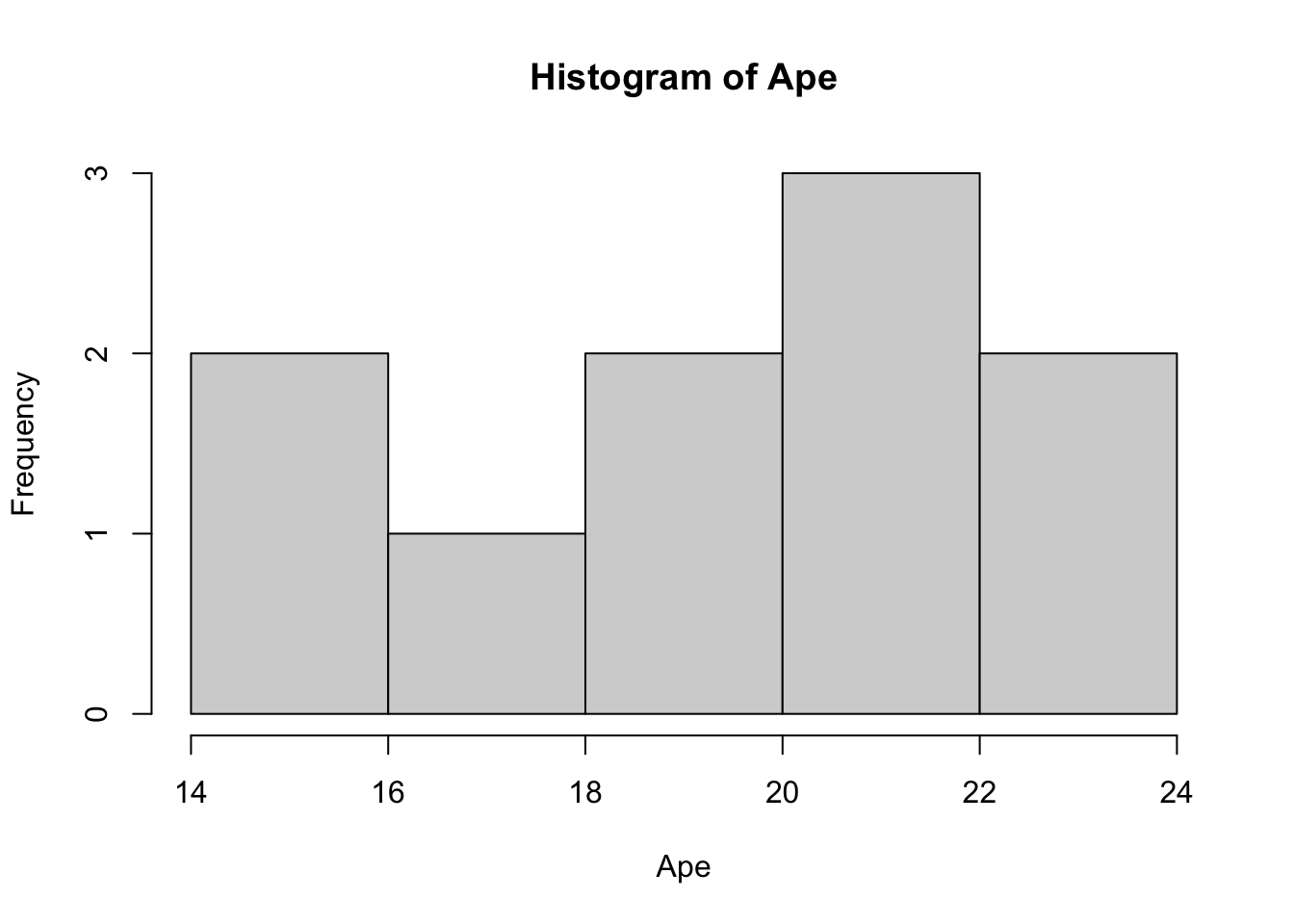
Figure 8.3: Histogram of Ape

While this sample may not look very Normal, we will soon see that we will not be able to give sufficient evidence to the contrary.

Taking the mean of the Ape vector gives us his average number of successes or repeated experiments.

mean( Ape )

## [1] 19.6

So, even though the mean isn’t 20, it is fairly close and this series of experiments does seem to simulate a BADR which would average 20 successes out of 40 over the long run.

Returning to our favorite little blonde girl, Melody, the reason we are even having this discussion was that her father, being a mathematician, kept track of how often she chose the correct feet for her shoes. A simple whiteboard was near their front door and her father would simply mark whether she had it right as they went to leave the house. This “experiment” showed that Melody had only put her shoes on the correct feet 13 out of 40 times. We can explore the unlikeliness of this with an exploration.

This exploration allows you to look at how often a sample of BADRs were as unlucky as Melody.

You can change the sample size by dragging the black dot along the horizontal line and get a new sample by dragging the Randomizer slider.

Further investigation can be done using these tools as well as the tools opened by toggling the “Advanced Tools” slider. (This slider is only available once the “Unlucky Region” slider is toggled to “On.”) However, we will not go further here. Reach out to your instructor or the author of Statypus if you have questions on what else you can do with this exploration.

We can use dbinom to find the exact probability of this result.

dbinom( x = 13, size = 40, prob = 0.5 )

## [1] 0.01094415

The probability that Melody should have had this low of a success rate as she did or worse would be found using pbinom.

pbinom( q = 13, size = 40, prob = 0.5 )

## [1] 0.01923865

Thus, our theoretical result is that the Melody should have only expected such poor results about 1.92% of the time.⁷⁷

Returning to our blind ape, let’s imagine that we place one million blind apes in dark rooms and let them attempt the shoe experiment with 40 trials each. We can simulate the proportion of BADRs that achieved less than or equal to 13 out of 40 successes using rbinom.⁷⁸

Apes <- rbinom( n = 1000000, size = 40, prob = 0.5 )
mean( Apes <= 13 )

## [1] 0.019304

This value of 1.93% is very close to what we found with pbinom and we remind the reader that running the above code again or on your own machine would give a different, yet similar result.

Plotting a histogram of the Apes data, using the code we first saw in Section 3.3.2, gives the following.

data <- Apes
bin_width <- 1
hist( 
      data, 
      freq = TRUE, 
      breaks = seq( 
                      from = min( data, na.rm = TRUE ) - 0.5, 
                      to = max( data, na.rm = TRUE ) + bin_width - 0.5, 
                      by = bin_width
                  )
    )

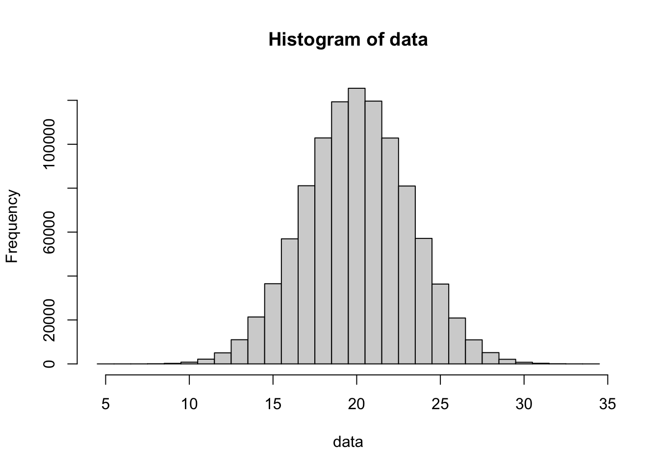
Figure 8.4: Histogram of Apes

This looks very similar to a Normal distribution and a Normal approximation can be used. In fact, the following is a graph of a perfectly Normal distribution with \({\mu = n p = 40 * 0.5 = 20}\) and \({\sigma = \sqrt{n p (1-p)} = \sqrt{40*0.5*0.5} = \sqrt{10} \approx 3.1623}\) overlayed on the above histogram.

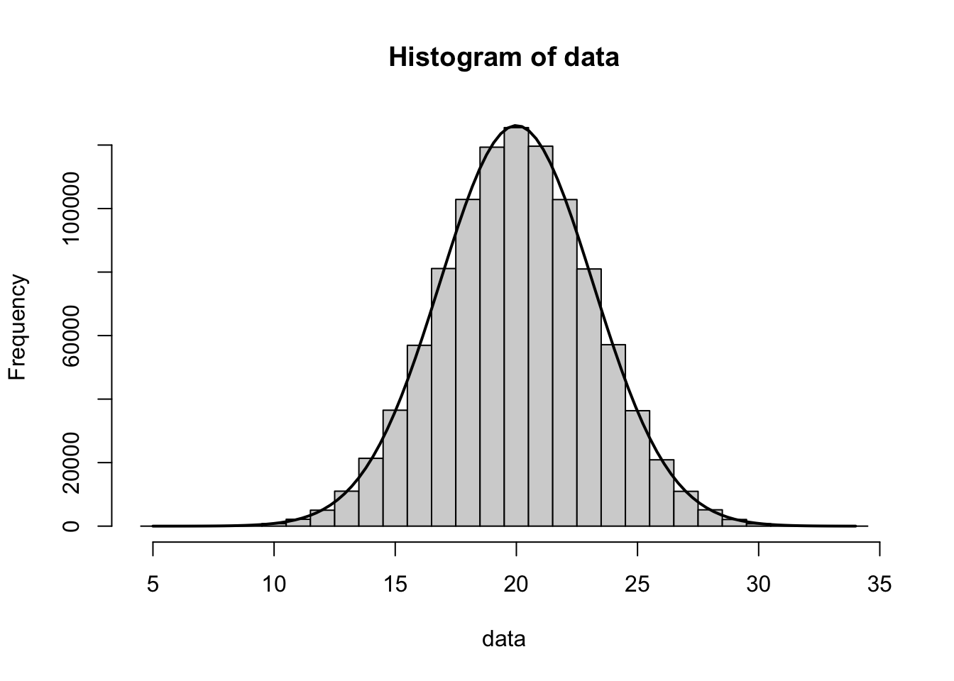
Figure 8.5: Histogram of Apes with Theoretical Model

This is a great motivating example to why the Normal approximation⁷⁹ can be used for the Binomial Distribution. It is also the backbone of the techniques we will use when we start doing inferential statistics with regards to a population proportion.

8.5 The Normal Approximation to the Binomial Distribution

Remark. This section is optional in some introductory statistics courses.

The Normal distribution can be used in many different applications. One such place is to approximate a Binomial distribution. It is worth noting that this section is thus offering an approximation for a distribution we just developed exact techniques for. This may seem silly, but does offer a nice transition to the concept of sampling distributions and gives rise to the formulas for the distribution of sample proportions.

8.5.1 The Normal Approximation

In order for the Normal distribution to be a suitable approximation to a Binomial distribution, we need that the number of expected successes and failures to both be at least 5.

Theorem 8.2 If we consider if individuals in a population of size \(N\) have a certain trait, we can use a Normal distribution to approximate binomial probabilities. More specifically, given a sample of size \(n\) from a population with a population proportion \(p\) such that \(n \cdot p \geq 5\), \(n \cdot (1-p) \geq 5\), and \(n << N\), the number of successes, \(X\), can be approximated as a random Normal variable with the following parameters.

\[\begin{align*} \mu_X & = n \cdot p\\ \sigma_X & = \sqrt{n \cdot p \cdot (1-p)} \end{align*}\]

8.5.2 Continuity Correction

One must be careful when using this approximation, however. If we return to the example of our Apes dataset that we first saw in Section 8.4, we can see that if we were to use this with the following methodology: \[P(X = n) \approx P\left( n-1 < X \leq n \right)\] then we would be doing the following approximation shown as the blue shaded area approximating the area of the rectangle it overlaps.

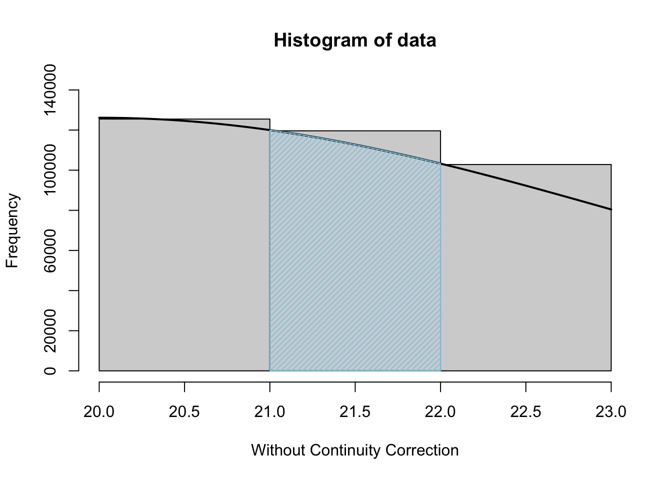
Figure 8.6: Normal Approximation without Continuity Correction

In this case, we are explicitly looking at the following.

\[P(X = 22) \approx P\left( 21 < X \leq 22\right)\] It is clear that this will always give rise to a lot of approximation error as we expect the Normal approximation to match the histogram data at the left hand upper corner of the rectangles. We can invoke the continuity correction where we instead use the methodology of:

\[P(X = n) \approx P\left( n - \frac{1}{2} < X \leq n + \frac{1}{2}\right)\] This shifts the portion of the Normal distribution that we use to the left by a half a unit which is equivalent to using the blue shaded area to approximate the rectangle it overlaps below.

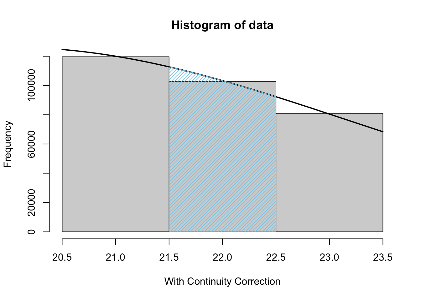
Figure 8.7: Normal Approximation with Continuity Correction

This gives an example of the approximations that would being made for each value of \(X\) in the Binomial Distribution.⁸⁰ It is clear that the continuity correction does offer a better approximation.

In this case, we were explicitly looking at

\[P(X = 22) \approx P\left( 21.5 < X \leq 22.5\right).\]

However, as we will be able to find exact values for Binomial and population proportion calculations, we will not focus much on this here. This technique is covered in many introductory statistics books, however, so the concept of a continuity correction is at least introduced.

Example 8.4 We can revisit the probability that a fair coin achieved between 22 and 28 heads inclusively. The code we used previously is shown below.

n <- 50
p <- 0.5
pbinom( q = 28, size = n, prob = p ) - pbinom( q = 21, size = n, prob = p )

## [1] 0.6777637

We compare this with the Normal Approximation code below.

mu <- n * p 
sigma <- sqrt(n * p * (1-p))
pnorm( q = 28.5, mean = mu, sd = sigma ) - pnorm( q = 21.5, mean = mu, sd = sigma )

## [1] 0.6778012

This is a very good approximation and one which we will leverage in the near future to analyze population and sample proportions.

Exercises

Exercise 8.1 Suppose a certain kitchen organizer requires a sliding rack to be attached to its base with 8 screws. Assume the probability that a random screw is usable is 0.999.

1. If the manufacturer only supplies 8 screws, what is the probability that all 8 screws will be usable?

2. If the manufacturer includes 9 screws, what is the probability that at least 8 of them will be usable?

3. If each customer who receives less than 8 usable screws returns the item, how many returns should the manufacturer expect per 1000 products sold if they provide only 8 screws? What if they provide an extra ninth screw? If the cost to the company for every return is $30, how much does the company expect to save per 1000 returns by including a ninth screw?
   

Exercise 8.2 Steph Curry⁸¹ has the highest lifetime free throw percentage in the NBA as of the writing of this document with a rate of 91.0%. If we assume that each of Steph’s free throw attempts is independent⁸², we can imagine Steph shooting 100 free throws as a Binomial experiment.

1. What is the probability that Steph makes exactly 91 out of 100 free throws?
2. What is the probability that Steph makes all 100 free throws?
3. What is the probability that Steph makes more than 95 free throws?
4. How many free throws does Steph have to make out of 100 to ensure he isn’t in the worst 1% of his attempts at 100 free throws?

Exercise 8.3 We return to Steph Curry and still assume that his population proportion for free throws is 91.0%. This means that we expect Steph to make at least 90% of his free throws, but how likely is that? We answer this with the following set of questions.

1. What is the probability that Steph makes at least 90% of his shots when shooting 10 free throws?
2. What is the probability that Steph makes at least 90% of his shots when shooting 100 free throws?
3. What is the probability that Steph makes at least 90% of his shots when shooting 1000 free throws?
4. What is the probability that Steph makes at least 90% of his shots when shooting 10000 free throws?

Exercise 8.4 What is the highest free throw percentage (to the nearest tenth of a percent) that a person (NOT Steph Curry) could have that would have a more than 1% chance of making 0 out of 100 free throws?

Exercise 8.5 If a student guesses randomly on an entire TRUE/FALSE test, it could be considered an example of a binomial experiment. If there are 50 TRUE/FALSE problems on test, what percentages of students should achieve a 70% or above on the test guessing randomly on all questions?

Challenge Problems:

Exercise 8.6 Be a critical consumer and/or statistician and explain how the logic in Example 8.2 in Section 8.3 may be inaccurate. For any critique offered, try to offer a suggestion on how we could attempt to correct our analysis.

Exercise 8.7 The actual origin of Example 8.2 in Section 8.3 and numerous problems here was was when the author was assembling a kitchen organizational product that required the installation of 8 thumb screws. Look online for the cost of thumb screws. (Buy in bulk to reduce costs.) What is a typical cost for 1000 thumb screws? At this cost, what level of precision does the thumb screw have to have before it is not cheaper to include an extra thumb screw if 8 good thumb screws are required? Assume the production cost of the product is $25 without an extra thumb screw.

Exercise 8.8 In Example 8.3, we investigated the concept of intentionally overbooking flights to guarantee the fullest possible flight. However, in that example, we did not account for the danger the airline risks of having to pay compensation to ticketed passengers who end up “overbooked,” i.e. who don’t have a seat.

Assuming we are dealing with a Boeing 737-800 in a one class configuration, we have 189 seats which can be sold to passengers. We will assume that each passenger’s decision to make or miss a flight is independent and that each passenger has a 5% chance of missing the flight. We will assume that the airline stands to make $200 for each passenger that actually takes a particular flight.

If the airline sells only 189 tickets, then they can expect approximately 5% of people to miss the flight. This is why airlines will intentionally “overbook” flights by selling more tickets than the number of available seats available.

1. If the airline sells exactly 189 tickets, find the expected revenue loss (that is the population mean of the discrete variable as defined in Section 6.2) for the airline compared to if the flight was full.

2. What is the expected number of missing passengers and how does this value compare to the value found in part a.?

3. What is the expected revenue loss if the airline sells 190 tickets if we assume that there is no penalty to the airline for an overbooked passenger other than the $200 that won’t be collected from the extra ticket?

The difference in the answers to parts a. and c. of this exercise is the revenue gain the company can expect if they sell an extra ticket.

4. What is the probability that all 150 ticketed passengers actually make the flight?

The airline will have to compensate anyone who is overbooked. If we multiply any compensation amount given to the overbooked passenger by the probability in part d. we get the expected loss encountered due to the overbooking.

5. If we divide the difference of the values in parts a. and c. by the probability in part d. we get the maximum compensation that the airline can give to an overbooked passenger and still expected a monetary gain if they sell 190 tickets. What is this value?

Warning: The following part is much harder.

6. If airlines should expect to pay the federal maximum of 400% of the one way ticket⁸³ in compensation to each overbooked passenger, how many extra seats should the airline sell to maximize profit?

Using the techniques we saw in Example 8.3, what is the probability that any passenger is overbooked if the airline sells the number of tickets found in park f.?

Exercise 8.9 Give reasons why the setup in Exercise 8.5 may not be a perfect binomial experiment.

8.6 Appendix

This appendix will expand on topics covered in this chapter and start to introduce topics found in Chapters 9 and 14. We begin by shifting our attention to random samples of 10 apes at a time and finding their sample means as values. This is done with the following code.

mean( rbinom( n = 10, size = 40, prob = 0.5 ) )

## [1] 20.8

This one sample of 10 blind apes shows a mean of 20.8 correct attempts out of 40, but each sample will likely differ. Replicating this one thousand times and looking at a histogram gives the following.

MeanApes <- replicate( 
                        n = 1000, 
                        {
                            mean( rbinom( n = 10, size = 40, prob = 0.5 ) )
                        }
                     )
hist( MeanApes )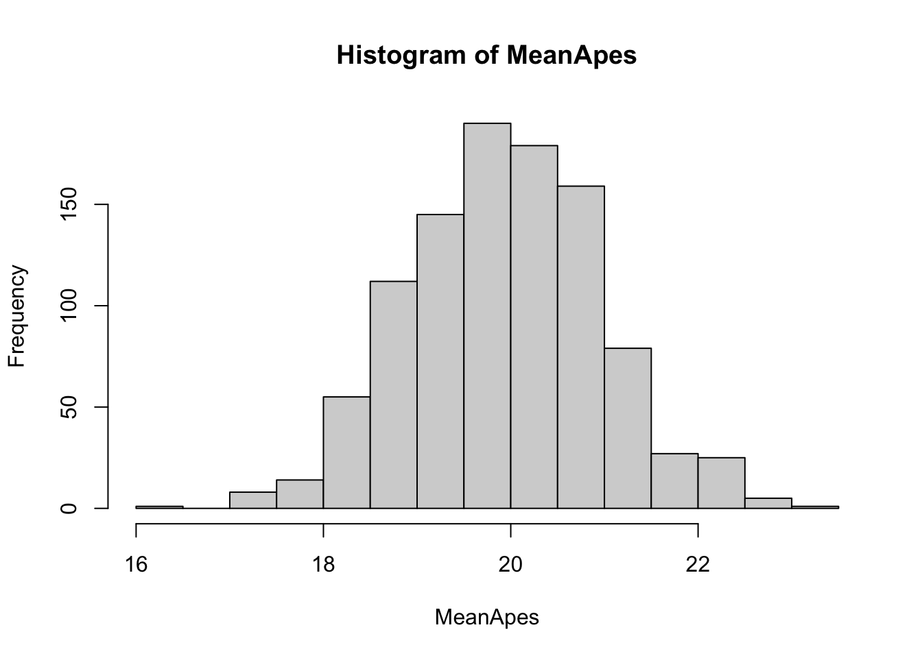

Figure 8.8: Histogram of MeanApes

We can overlay this with the projected distribution it should be in (which we do not yet have the formulas for) below.

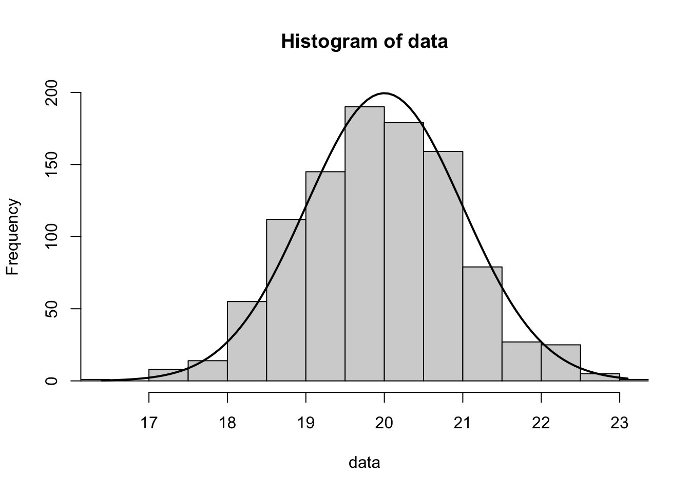
Figure 8.9: Histogram of MeanApes with Theoretical Model

While this may not appease our senses as much as that of Apes, the curious reader can run a QQ analysis and find that Apes would indicate that its underlying population is not Normal, while MeanApes would not indicate such.⁸⁴ Below is the code to run the QQ analysis on MeanApes.

x <- MeanApes      #This is either the vector name or of form df$colName
length( x )

## [1] 1000

QQ <- qqnorm( x )
qqline( x )

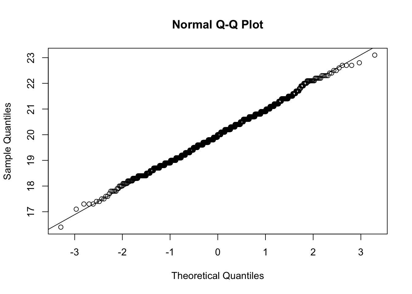
Figure 8.10: QQ Plot for MeanApes

cor( QQ$x, QQ$y )

## [1] 0.998827

This analysis confirms that we could not argue that MeanApes comes from a distribution that is not Normal. The QQ plot looks very straight and the r value of 0.998827 is well above either critical value found on the NIST table.⁸⁵

One reason to make sense of this is that the values in Apes can only take on whole number values while the values in MeanApes will typically have one decimal point.⁸⁶ The smoothness of the histogram for Apes is also due to the fact that we had one million apes in it as compared to only one thousand (maximal size we can test with the NIST table) groups of ten apes in MeanApes.

This little deviation from the individual values of Apes is a motivating example to show the power of sampling distributions. This is a technique that is heavily leveraged when we get to inferential statistics starting in Chapter 9.

---

69. November 2020, Mindy Weisberger-Senior Writer 02 (2 November 2020). “Platypuses glow an eerie blue-green under UV light”. livescience.com.↩︎

70. Jacob Bernoulli contributed significantly to the field of probability. In particular, in 1713 he proved his “Golden Theorem” which eventually became the first version of The Law of Large Numbers.↩︎

71. The very careful reader may also notice that this definition of the quantile function actually does not align with the definition of qdist we gave in Section 6.5 and this difficulty stems from the the incompatibility of making a bijection between a discrete set and the interval \([0,1]\). Cantor’s Diagonal Argument gives what is likely the easiest way to see the incompatibility of the natural numbers and the unit interval.↩︎

72. Since the quantities in the Binomial Distribution are discrete, we are able to use sum like we did here. However, for any quantity, \(x_0\), in a Normal distribution, we get that \(P(X = x_0) = 0\) and as such, we can not use the sum idea in that instance. Certain readers may recognize that the concept of a definite integral would be what is needed to go from the probability density function to the cumulative distribution function for a Normal distribution, but that technique is beyond the scope of this course.↩︎

73. The modern emergence of companies like Amazon have fundamentally changed the marketplace when it comes to returns. These types of companies have made it very easy to return defective products to ensure customer satisfaction and optimize customer loyalty.↩︎

74. A lot of companies now include a statement in some products asking the consumer to conduct them for questions about assembly or if any pieces are missing. This is done to drive down the number of returns as well. It is likely cheaper to mail a consumer a new screw or even entire hardware kit than it is to fully refund the customer or offer a replacement.↩︎

75. See Wikipedia for more information about the Boeing 737-800.↩︎

76. There is a very nice “redemption arc” to this story. However, the culmination of this story won’t be revealed until Chapter 9. We encourage the reader to stay tuned for that.↩︎

77. We are using the assumption that each of Melody’s attempts is independent, but there are many arguments for why this wasn’t the case. However, the author is very partial to this story and it is used at least as an allegorical/motivational example.↩︎

78. The technique used here was developed in Section 6.3, but that topic is optional and not covered in all sections.↩︎

79. The dnorm() function was not introduced in Chapter 7, but it is the Probability Density Function for the Normal Distribution. It’s use for actually computing probabilities would require the calculus concept of definite integration. The curious reader can run ?integrate and look at the examples given.↩︎

80. For those readers who have taken calculus, it is an interesting note that in this situation we are using an integral as an approximation of a rectangle as compared to the other way around.↩︎

81. See Wikipedia for more information.↩︎

82. The Hot Hand Phenomenon or Hot Hand Fallacy is a theory surrounding precisely the independence of subsequent athletic endeavors such as free throw shooting. There have been numerous research articles on the topic, and one from January 2022 can be found at https://doi.org/10.1371/journal.pone.0261890 and the datasets analyzed can be found at https://github.com/kpelechrinis/HotHand-NBA-Tracking.↩︎

83. See this LINK for more information.↩︎

84. See Chapter 14 for a full discussion on QQ analysis.↩︎

85. The table can be found at https://www.itl.nist.gov/div898/handbook/eda/section3/eda3676.htm.↩︎

86. The curious reader is encouraged to investigate this further. The author only achieved values of r near 0.9958 for Apes.↩︎