Chapter 10 Inference for Population Mean(s)

Figure 10.1: A Statypus Taking Pride in their Name
The platypus does not have teeth (at least as an adult) nor a traditional stomach. They do have a small pouch which has a similar function to our stomachs, but it does not use acids or digestive juices to break down food. Due to these oddities, a platypus will often swallow small pebbles (is that a calculus?166) to help them crush and break down their food.167
In Chapter 9, we looked at the techniques for doing inferential statistics on a population proportion. This typically occurs when one is looking at qualitative data as it is easy to ask “What proportion of a population has a certain value of the given qualitative variable?” In our example, one example we looked at was what proportion of M&Ms had a certain color.
However, if we want to understand quantitative data, we might want to study the population mean of a certain variable. The techniques in this chapter will allow us to infer information about a population mean parameter only from a sample mean statistic. For example, someone may want to know the population mean for the weight of all babies born. However, this value would be nearly impossible to gather exactly as it would require the knowledge of the weight168 of every baby ever born and the value would, in theory, change with each new birth. However, the aim of this chapter will be to gather as much information about the population mean weight of babies at birth using samples such as those we saw in Chapter 7.
New R Functions Used
Most of the functions listed below have a help file built into RStudio. Most of these functions have options which are not fully covered or not mentioned in this chapter. To access more information about other functionality and uses for these functions, use the ? command. E.g. To see the help file for qnorm, you can run ?t.test or ?t.test() in either an R Script or in your Console.
We will see the following functions in Chapter 10.
pt(): Distribution function for the \(t\) distribution withdfdegrees of freedom.t.test(): Performs one and two sample t-tests on vectors of data.qt(): Quantile function for the \(t\) distribution withdfdegrees of freedom.ConfIntFromSample(): Compares the middle values of a sample to the obtained confidence interval. [Statypus Original Function]
ConfIntFromSample() was developed at Saint Louis University and does not have any built in help file. Please see Section 10.5.2 if you have further questions about its functionality.
To load all of the datasets used in Chapter 10, run the following line of code.
10.1 Part 1: Distribution of Sample Means
The key tool we will use to understand the distribution of sample means is the Central Limit Theorem, first introduced in Chapter 9.
Theorem 9.1 \(\;\) Given a distribution or random variable, \(X\), with a population mean of \(\mu_X\) and a population standard deviation of \(\sigma_X\), then the collection of samples of size \(n\) gives rise to a distribution of sample means, \(\bar{x}\), which have mean and standard deviation given below. \[\begin{align*} \mu_{\bar{x}} & = \mu_X\\ \sigma_{\bar{x}} & = \frac{\sigma_X}{\sqrt{n}} \end{align*}\]
If the original distribution was Normal, then the distribution of sample means is also Normal.
However, the distribution approaches Norm\((\mu_{\bar{x}}, \sigma_{\bar{x}})\) as \(n\) gets large regardless of the shape of the original distribution.
A great video by 3Blue1Brown is shown below discussing the Central Limit Theorem.
Example 10.1 To visualize the last part of the CLT, we will use one million rolls of a standard 6 sided die as our original distribution. Below is a histogram of one million random dice rolls which approximates the (uniform) distribution. We found that \(\mu_X = 3.5\) for a fair die in Example 6.5.
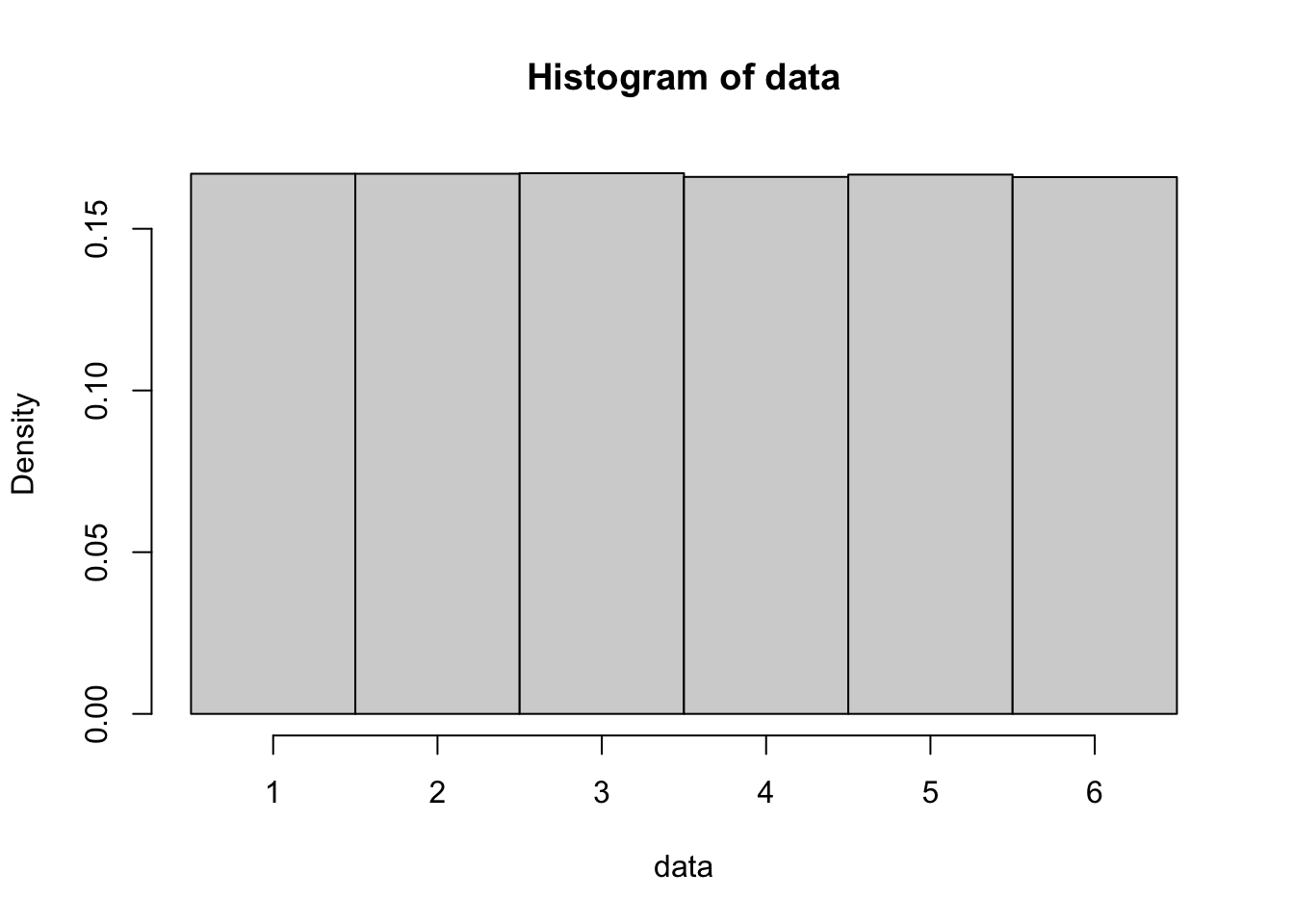
Figure 10.2: Histogram of One Million Rolls of a Single Die
If we shift to now doing sample means, we begin with the simplest case, which is the mean of two dice rolls. Here we roll 2 dice a total of ten thousand times and find the mean of the two dice.
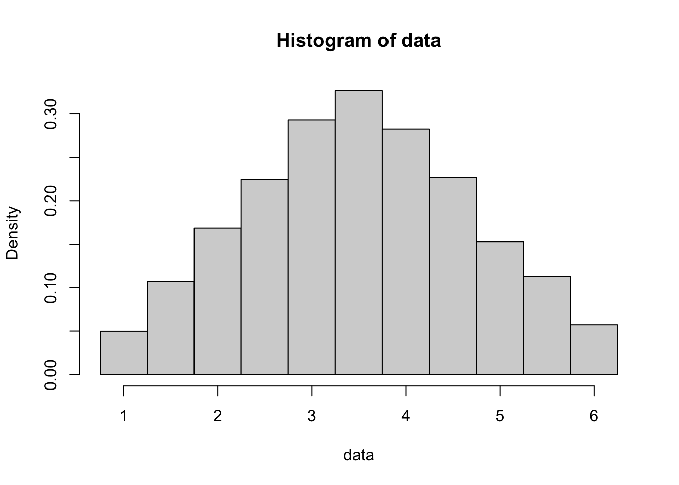
Figure 10.3: Histogram of Ten Thousand Rolls of a Pair of Dice
While the histogram still ranges from 1 to 6, the distribution is clearly more centralized around 3.5. This histogram is triangular rather than bell shaped. The familiar bell shape will emerge as we increase the number of dice we roll each time, which we call the value of \(n\).
If we now move to a sample size of \(n = 5\), we get the following histogram and theoretical distribution after one hundred thousand rolls of 5 dice.

Figure 10.4: Histogram of Ten Thousand Rolls of Five Dice
The range of the distribution is still the same, but we again see an even larger grouping of values near \(\bar{x} = 3.5\) and start to see the familiar “bell” shape we are expecting from a Normal distribution.
Moving to \(n = 100\) gives the following graph which looks nearly perfectly Normal and centered at \(\bar{x} = 3.5\).
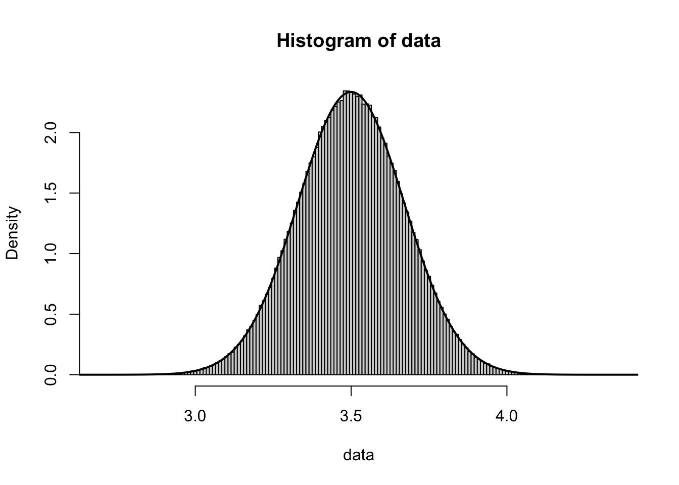
Figure 10.5: Histogram of Ten Thousand Rolls of One Hundred Dice
Analysis of \(\sigma_{\bar{x}}\) would require us to know the value of \(\sigma_X\). In Example 6.5, we showed that
\[\sigma_X = \sqrt{\frac{35}{12}}\approx 1.708\]
which gives (approximate) values of 1.208, 0.764, and 0.171 for \(\sigma_{\bar{x}}\) for \(n = 2, 5, \text{and }100\).
The value \(\sigma_{\bar{x}} \approx 0.171\) visually matches the above graph very well when looking at the distance from the center of the graph to the inflection points (as we did in the Exploration right before Theorem 7.1).
The following exploration can be used in conjunction with or in lieu of Example 10.1.
This simulation shows a simulation of a large number of dice. The green Sample Size slider dictates how many dice are rolled at a time and the data in the histogram is then the mean value of those dice rolls. The purple “Show Model” slider can be used to toggle on the theoretical model for a histogram of this data.
Keeping the Sample Size at 1, adjust the orange slider to see other large samples of dice rolls. You should see a nearly uniform distribution which looks nothing like a bell curve.
Adjusting the Sample Size to be 2, the histogram should now appear to be triangular rather than uniform or bell shaped. Adjusting the orange slider will give other histograms which should closely resemble the theoretical model which can be seen by toggling the purple “Show Model” slider.
Adjusting the Sample Size to a value higher than 2, we see that the distribution now resembles a bell curve and this is what is shown with the purple “Show Model” slider.
Increasing the Sample Size also affects the “width” of the model shown where it begins by spanning the entire range of 1 to 6 and then begins becoming more centralized around 3.5.
Note: Unfortunately, due to Desmos memory limits, the in-house Statypus coder was unable to achieve a large enough number of samples if the sample size was greater than 6. Look at Example 10.1 to see what happens if we increase the sample size well beyond 6.
Example 10.2 (Samples Versus Individuals) In Example 7.3, we claimed that the distribution of heights of US adult men was approximately \(\text{Norm}(69,3)\). Using the Empirical Rule (see Section 7.5 if needed), we can say that approximately 95% of US adult men have a height within 2 population standard deviations of the population mean. That is, we expect that approximately 95% of US adult men to have a height between \(69 - 2\cdot 3 = 63\) and \(69 + 2\cdot 3 = 75\) inches. To put that into simpler English, approximately 95% of US adult men will stand between 5 foot 3 inches tall and 6 foot 3 inches tall. This also means that if we had a room of 25 US adult males, that we would expect at least one person (\(0.05 \cdot 25 = 1.25\)) to have a height that is outside of that range.
However, if we considered a room of 25 US adult males as an SRS from the population, then we expect that the mean height of the room should follow the \(\text{Norm}\left( 69, \frac{3}{\sqrt{25}}\right) = \text{Norm}\left( 69, \frac{3}{5}\right)\) distribution. That is, we expect approximately 95% of samples of 25 US adult males to have a sample mean height between \(69 - 2\cdot \frac{3}{5} = 67 \frac{4}{5}\) and \(69 + 2\cdot \frac{3}{5} = 70\frac{1}{5}\) inches. That is to say that 95% of samples would have a mean that falls between 5 foot \(7\frac{4}{5}\) and 5 foot \(10 \frac{1}{5}\) inches tall.
To put this in perspective, the probability that a random US adult male would be at least 6 foot (72 inches) tall can be found with the following code.
## [1] 0.1586553This says that roughly 15.9% of US adult males are at least 6 foot tall.
However, if we consider samples of 25 US adult males, then the probability that a random sample would have a sample mean at least 6 foot would be given by the following code where we set sd = 3 / 5 based on the Central Limit Theorem.
## [1] 2.866516e-07This is a much smaller number! Taking the reciprocal, we can say that we should only expect an SRS of 25 US adult males to have a mean height of at least 6 foot once in every roughly 3.5 million samples!
## [1] 3488556We know that IQ scores roughly follow \(\text{Norm}(100,15)\).
Using the Empirical Rule, answer the following questions.
- Approximately what proportion of people will have an IQ between 85 and 115?
- Approximately what proportion of samples of \(n=4\) people (thought of as families) have a mean IQ between 85 and 115?
Using R functions, answer the following questions.
- What proportion of people will have an IQ over 120?
- What proportion of samples of \(n=4\) people have a mean IQ over 120?
- What proportion of samples of \(n=25\) people (thought of as a class of kids) have a mean IQ lower than 70?
Exercises
Exercise 10.1 Assuming that the heights of US adult females follow \(\text{Norm}(64.5, 2.5)\), answer the following questions.
- What proportion of US adult females are shorter than 5 foot 4.5 inches?
- What proportion of samples of size \(n=10\) US adult females have a sample mean shorter than 5 foot 4.5 inches?
- What proportion of US adult females are taller than 5 foot 6 inches?
- What proportion of samples of size \(n=10\) US adult females have a sample mean taller than 5 foot 6 inches?
- What proportion of US adult females are between 5 foot 4 inches and 5 foot 7 inches?
- What proportion of samples of size \(n=20\) US adult females have a sample mean between 5 foot 4 inches and 5 foot 7 inches?
Exercise 10.2 ACT Scores are approximately normal with \(\mu = 21\) and \(\sigma = 5\). Using these values, answer the following questions.
- What is the probability that a random student will score higher than a 22 on the ACT?
- What is the probability that a random sample of \(n=25\) students (a single AP Bio class) will achieve a mean higher than 22 on the ACT?
- What is the probability that a random sample of \(n=400\) students (an entire Senior class) will achieve a mean higher than 22 on the ACT?
10.2 Part 2: Hypothesis Tests for a Population Mean
In our derivation of the hypothesis test for a population proportion, we used a statistic, \(\hat{p}\), to make a decision about the value of a parameter, \(p\). We now want to do this again but now use \(\bar{x}\) (and \(s_{\bf x}\)) to infer information about \(\mu\).
We begin by reminding ourselves of the steps involved in conducting a hypothesis test.
In order to prove a statistical claim, we will follow the same steps as in a criminal court case.
Step 1: A researcher (prosecutor) must choose to investigate a certain concept.
Step 2: After possibly a cursory investigation, the researcher must formally make a claim.
Step 3: The researcher then must gather evidence surrounding their claim.
Step 4: IF the evidence gathered supports their claim, then they can move to test the claim (have a trial).
Step 5: All calculations (proceedings) must be conducted under the strict assumption that our claim is false (the defendant is innocent).
Step 6: After all evidence has been examined (under the assumptions in Step 5), it must be decided if it can be believed that the evidence supporting the claim can be attributed to chance alone.
Outcome 1: If the evidence is not compelling enough, we must choose to stand by our assumption and decide that the claim cannot be proven despite the evidence supporting it (finding the defendant not-guilty).
Outcome 2: If the evidence is compelling enough, we can choose to reject our assumption and say that we have proven the claim (found the defendant guilty)To move further, we must know the type of statements that we will be testing.
Following in the mindset from Chapter 9, we are looking to conduct a test between hypotheses of form
\[\begin{align*} H_0 &: \mu = \mu_0\\ H_a &: \mu\; \Box \;\mu_0 \end{align*}\]
where \(\Box\) can be one of the symbols: \(\neq\), <, or >.
Like in Section 9.3.2, we will adopt the mentality that prior to analyzing the evidence, that we have assumed \(H_0\) and thus believe it 100%. However, we will loosely interpret the \(p\)-value as our belief in \(H_0\) after we have analyzed the evidence we found from the data.169
In our derivation of the \(p\)-value in Section 9.3.3, we used a \(z\)-statistic (zStat within R code). Here we want to use the fact that \(\bar{x}\) is the point estimate of \(\mu\) and the results of the Central Limit Theorem, Theorem 9.1.
\[\begin{align*}
\mu_{\bar{x}} &= \mu_X\\
\sigma_{\bar{x}} &= \frac{\sigma_X}{\sqrt{n}}
\end{align*}\]
We will conduct our investigations starting with the assumption that we know the value of \(\mu_X\), but it is helpful to remember that we actually are trying to infer information about the value of \(\mu_X\). If we do not have information about \(\sigma_X\) we will be forced to use the approximation that \(\sigma_X \approx s_{\bf x}\). If we had \(\sigma_X\), or \(\sigma_{\bar{x}},\) then we could use the \(z\)-distribution. However, if we substitute in \(s_{\bf x}\) for \(\sigma_X\) when standardizing our data, the resulting distribution isn’t Normal.
Some textbooks do give a process for using the \(z\)-distribution to perform hypothesis testing and construct confidence intervals for a population mean when the population standard deviation, \(\sigma_X\), is known. However, we omit this process here on Statypus and focus on the situation where we are forced to use the sample standard deviation.
10.2.1 Student’s t-distribution
We can save the method shown above by offering a generalization of the \(z\)-distribution, which is Student’s \(t\)-distribution. To motivate this, we can look at some simulated data. We collect 100,000 samples of size \(n=4\) of individuals from a known Normal distribution, \(\text{Norm}( \mu_X, \sigma_X)\). For each sample, we calculate the following standardized value.
\[z = \frac{\bar{x} - \mu_{\bar{x}}}{\sigma_{\bar{x}}} =\frac{\bar{x} - \mu_X}{\left( \frac{\sigma_X}{\sqrt{n}} \right)}\] We can then construct a histogram of the 100,000 values of \(z\) and superimpose the Standard Normal Distribution over it.
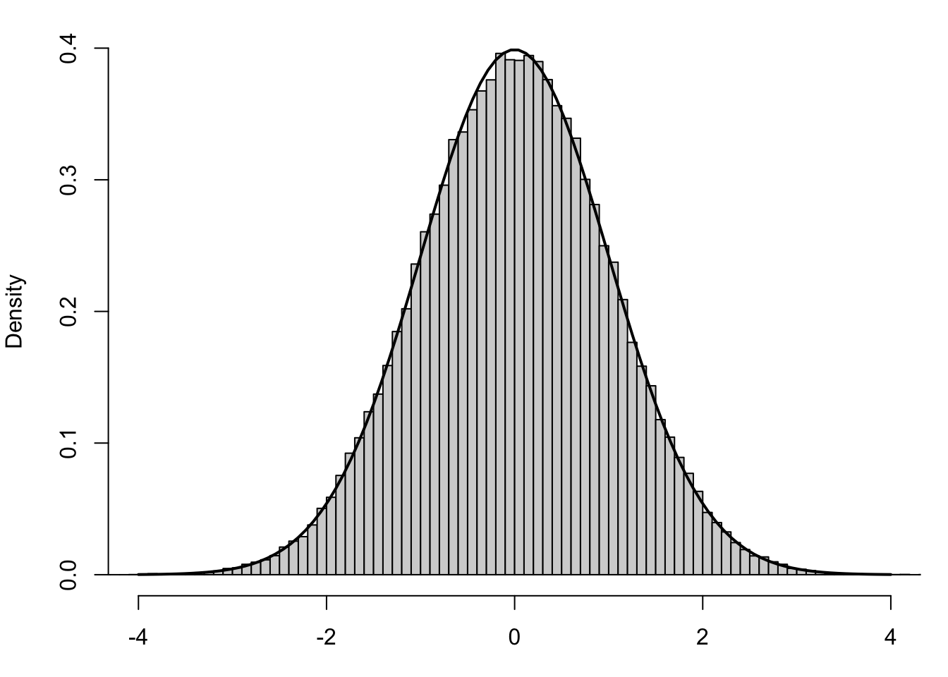
Figure 10.6: Standardized Values using Population Standard Deviation
This shows that the values of \(z\) are very well modeled by the Standard Normal Distribution. However, what happens if we don’t know \(\mu_X\) and are forced to make the following approximation?
Definition 10.1 Given a sample of size \(n\), we will say the Standard Error of the sample is given by
\[\text{SE} = \frac{s_{\bf x}}{\sqrt{n}}.\]
Like in Chapter 9, we have that the Standard Error is our point estimate for the standard deviation of the distribution of the sample statistic. In this case we have that
\[\text{SE} \approx \sigma_{\bar{x}}\]
or that
\[\frac{s_{\bf x}}{\sqrt{n}} \approx \frac{\sigma_X}{\sqrt{n}}.\]
This leads to the following approximation in the following formula used for \(z\) above.
\[\frac{\bar{x} - \mu_0}{\left(\frac{s_{\bf x}}{\sqrt{n}}\right)} \approx \frac{\bar{x} - \mu_0}{\left(\frac{\sigma_X}{\sqrt{n}}\right)} = z\] The result is our analog of the \(z\)-statistic from Section 9.3.3 and is what we will call the \(\bf t\)-statistic.
Definition 10.2 Given a sample of values, with a sample mean of \(\bar{x}\), from a population assumed to have a population mean of \(\mu_0\), the test statistic associated to the sample is now referred to as the \(\bf t\)-statistic and is found via the formula below
\[ t = \frac{ \bar{x}_0 - \mu_0}{\left(\frac{s_{\bf x}}{\sqrt{n}}\right)}\]
where \(s_{\bf x}\) is the sample standard deviation of the sample and \(n\) is the sample size.
The structure is identical to that of the standardized value of \(\bar{x}\), as defined in Section 4.4.3, save for the \(s_{\bf x} \approx \sigma_X\) approximation. We should now rightfully ask if the \(t\)-statistic is also Normally distributed. However, below is the same set of samples along with the Standard Normal Distribution.
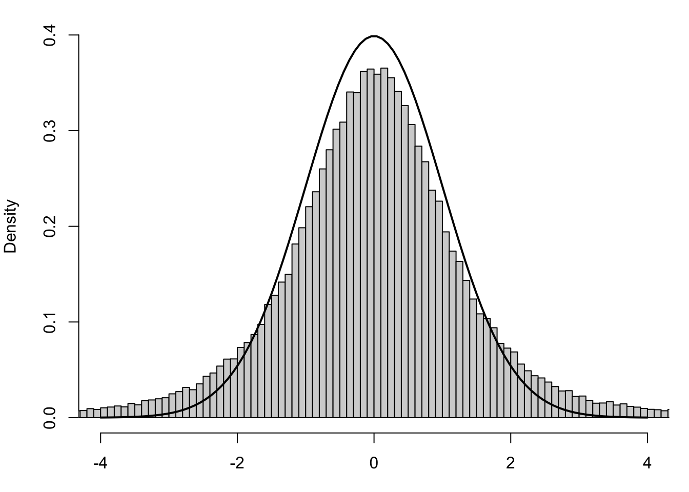
Figure 10.7: Standardized Values using Sample Standard Deviation
The black curve is still the Standard Normal Distribution, or \(z\)-distribution, and we see that the histogram now does not align well with it. If the values of \(t\) were to fit to the \(z\)-distribution, we wouldn’t have used a new letter for them. This leads to the following definition.
Definition 10.3 For a given value \(\nu \in \left[ 1, \infty\right)\), there is a continuous density function which generalizes the Standard Normal Distribution known as Student’s170 \(t\)-distribution.171 The parameter \(\nu\) (the Greek letter “nu”) is known as the Degrees of Freedom of the distribution.
Student’s \(t\)-distribution has “heavy tails”172 compared to the Standard Normal Distribution. However, as \(\nu\) gets large, Student’s \(t\)-Distribution becomes very similar to the Standard Normal Distribution. We will look at this shortly.
One key difference of \(t\) compared to \(z\) is that there is a different \(t\)-distribution for each degree of freedom. Recall that when we introduced a sample standard deviation that a sample of size \(n\) had \(n-1\) degrees of freedom and we used that when we set
\[ s_{\bf x} = \sqrt{\frac{\sum (x - \bar{x})^2}{n-1}}.\]
Student’s \(t\)-distribution uses this same value, \(\nu = n-1\), as the degrees of freedom when working with samples of size \(n\).173
When we have a degree of freedom equal to 1, Student’s \(t\)-distribution is what is known as the Cauchy Distribution. The Cauchy Distribution is shown below as the shaded blue graph while the black curve is the Standard Normal Distribution, or \(z\)-distribution.
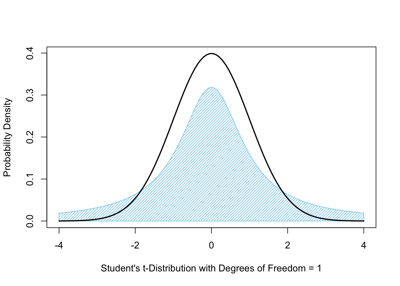
Figure 10.8: Student’s \(t\)-Distribution with 1 Degree of Freedom
In Figures 10.8 (above) and 10.9 (below), we show the area bound by \(t\)-distribution as compared to just the density function itself.
Increasing the degrees of freedom to 4 gives the following graph in blue, where, again, the black curve is the \(z\)-distribution.
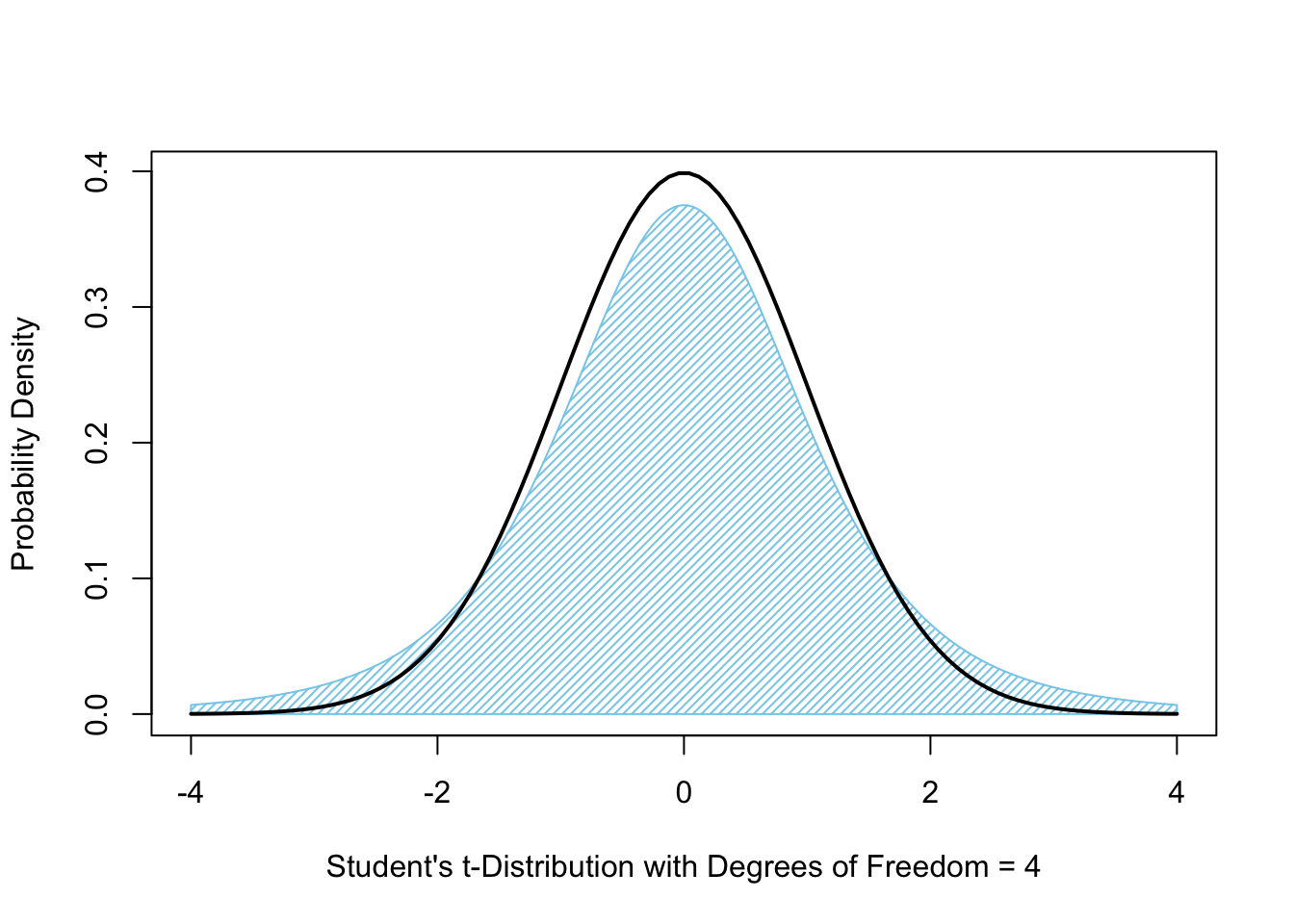
Figure 10.9: Student’s \(t\)-Distribution with 4 Degrees of Freedom
From here, it may be obvious that the \(t\)-distribution is approaching the \(z\)-distribution, but it is unsure if it will get there or even possibly overshoot it. It is true that as \(n\) gets larger that the \(t\)-distribution approached the \(z\)-distribution and as \(n\) gets large enough, they become nearly indistinguishable.174 That is, the \(t\) and \(z\) variables are roughly equivalent for large samples, but the \(t\)-distribution offers a bit of correction for small samples due to the inaccuracy of approximating \(\sigma_X\) with \(s_{\bf x}\).
If we revisit Figure 10.7 and further superimpose Student’s \(t\)-Distribution with 3 (one less than the sample size) degrees of freedom in blue, we get the following output which shows a much better fit.
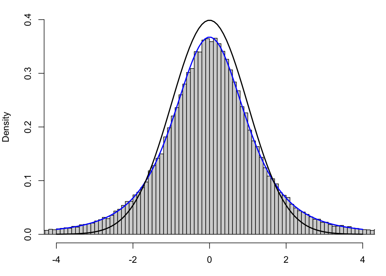
Figure 10.10: Standardized Values using Sample Standard Deviation
The \(t\)-distribution still has a noticeably positive value at \(t = \pm 4\) when the \(z\)-distribution is essentially 0 for values outside of \(z = \pm 4\). This is an example of what we mean by saying that Student’s \(t\)-Distribution has “heavy tails.”
The curious reader can investigate the structure of Student’s \(t\)-Distribution using the following Desmos Exploration.
The vertical Sample Size slider can be used to adjust the value of the degrees of freedom. As you increase this value, the \(t\)-distribution approaches the more familiar Standard Normal Distribution shown in black.
Further investigation can be done using these tools as well as the tools opened by toggling the other two sliders. However, we will not go further here. Reach out to your instructor or the author of Statypus if you have questions on what else you can do with this exploration.
The value of \(\frac{s_{\bf x}}{\sqrt{n}}\) is the Standard Error we introduced in Section 10.3. While we are assuming we know the value of the population mean, we have no information about the population standard deviation, \(\sigma_x\), and thus are forced to make the same approximation we did when constructing confidence intervals.
To make sense of this, let’s look at an example.
Example 10.3 We begin by importing the dataset PlatypusData1 from Statypus.
Use the following code to download PlatypusData1.
We will focus on only the female platypuses, so we start by extracting the values we wish to deal with.
We are curious if the mean weight of a female platypus is less than 1 kilogram. That is, we have that \(\mu_0 = 1\) and have the following set of Hypotheses:
\[\begin{align*} H_0 &: \mu = 1\\ H_a &: \mu < 1 \end{align*}\]
We can now adapt part of the code we developed in Example 10.9 now using tStat with its formula in lieu of the tStar we used for a confidence interval.
#Enter the data vector here
x =      FemalePlatys
#The value in the null hypothesis
mu0 =    1
#Number of tails
Tails =  1
#Nothing below needs altered
#Below here is stock code and should not be changed
x <- x[!is.na(x)]
xBar0 <- mean(x)           #Sample Mean
s <- sd(x)                 #Sample Standard Deviation
n <- length(x)             #Sample Size
SE <- s / sqrt( n )        #Standard Error
tStat <- (xBar0 - mu0)/SE  #t statistic
tStat
## [1] -4.752479In Section 9.3.3 we used the function pnorm, the distribution function for Normal variables, to convert zStat into a \(p\)-value. Now that we have shifted our attention to Student’s \(t\)-distribution, we need the analog, pt().
10.2.2 pt function
The pt() is the distribution function for Student’s \(t\)-distribution. We defined what a distribution function is in Section 6.5.2. The input is a quantile, q and the output is either \(P(t \leq q)\) or \(P( t > q)\) based on the choice of the argument lower.tail.
See Section 6.6 if you need a quick refresher on the distinction between distribution functions and quantile functions.
The syntax of pt() is
where the arguments are:
q: The quantile that sets \(P(t \leq q)\) or \(P( t > q)\).df: Degrees of freedom. It must be positive but may be a non-integer.df = Infis allowed.lower.tail: This option controls whether the quantity returned is an upper or lower bound. Iflower.tail = TRUE(orT), then the output is the probability \(P( t \leq q ) = p\). Iflower.tailis set toFALSE(orF), then the output is the probability \(P( t > q ) = p\). If no value is set, R will default tolower.tail = TRUE.
Example 10.4 We can now find the \(p\)-value associated to FemalePlatys by running the following line of code where the values of n and tStat are carried over from Example 10.3.
## [1] 3.372064e-06With a \(p\)-value of less than 0.0000034, we have sufficient evidence at any reasonable level of significance to reject the null hypothesis and can accept that claim that the mean mass of a female platypus is less than one kilogram.
10.2.3 Hypothesis Tests By Hand
We can combine the code developed so far in Section 10.2 to get the following.
To conduct a hypothesis test for a population mean “by hand,” use the following Code Template.
#Enter the data vector here
x =
#The value in the null hypothesis
mu0 =
#Number of tails
Tails =
#Nothing below needs altered
x <- x[!is.na(x)]
xBar0 <- mean(x)           #Sample Mean
s <- sd(x)                 #Sample Standard Deviation
n <- length(x)             #Sample Size
SE <- s / sqrt( n )        #Standard Error
tStat <- (xBar0 - mu0)/SE  #t statistic
pValue <- Tails * pt( q = - abs( tStat ), df = (n-1) )
pValue                     #p-Value
While the result of the above Code Template will only display the \(p\)-value, the values of all interim calculations are saved to your environment. For example, if you want to find the \(t\)-statistic, you can simply run the line
assuming you haven’t run any other code to rewrite the value tStat.
Example 10.5 Suppose you wanted to test if the mean birth mass of babies is 3200 grams. That is, we want to peform the following hypothesis test.
\[\begin{align*} H_0 &: \mu = 3200\\ H_a &: \mu \neq 3200 \end{align*}\]
We can use BabyData1$weight as our data which we introduced in Chapter 7.
Use the following code to download BabyData1.
We rebuild the “by hand” technique we developed for inferences about a population proportion by changing out the applicable values in the code. We use a t-score and also leverage the pt() function, which we just introduced, rather than the pnorm() function. In addition, as our null hypothesis, \(H_0\), is \(\mu \neq 3200\), we set Tails to be 2.
#Enter the data vector here
x = BabyData1$weight
#The value in the null hypothesis
mu0 = 3200
#Number of tails
Tails = 2
#Nothing below needs altered
x <- x[!is.na(x)]
xBar0 <- mean(x)           #Sample Mean
s <- sd(x)                 #Sample Standard Deviation
n <- length(x)             #Sample Size
SE <- s / sqrt( n )        #Standard Error
tStat <- (xBar0 - mu0)/SE  #t statistic
pValue <- Tails * pt( q = - abs( tStat ), df = (n-1) )
pValue                     #p-Value
## [1] 0.04104805This gives a \(p\)-value of 0.041 and if we select the \(\alpha = 0.05\) significance level, then our “belief in \(H_0\),” the \(p\)-value, has fallen below the acceptable threshold, \(\alpha\). Thus we can no longer “believe” \(H_0\) and can state that we have sufficient evidence to reject \(H_0\) and can accept \(H_a\) which states that \(\mu \neq 3200\).
10.2.4 t.test Saves the Day
Here is where our reliance on RStudio really begins to pay off. The calculations made above are a very fundamental part of inferential statistics and R has robust support of them. In Chapter 9, we initially used by hand calculations because the methods given by most introductory textbooks are based off approximations that were used to minimize the computational complexity but are simply not necessary with modern computers.
RStudio can do all of the above calculations for us and give us output which mirrors that which we saw in binom.test. The function we need here is t.test() and it will also give us a very natural nudge towards confidence intervals.
The syntax of t.test() is
#This code will not run unless the necessary values are inputted.
t.test( x, conf.level, mu, alternative )
where the arguments are:
x: The data vector we are using for inference.conf.level: The confidence level for the desired confidence interval. Not needed for hypothesis test.mu: The assumed value of \(\mu_X\) in the null hypothesis. Not needed for confidence intervals.alternative: The symbol in the alternative hypothesis in a hypothesis test. Must be one of"two.sided","less", and"greater". DO NOT USE for confidence intervals.
Example 10.6 With the power of t.test, we can redo the work of Example 10.5 with just one line175 of code. We now only need to implement the arguments mu and alternative just like we did with binom.test in Chapter 9.
##
##  One Sample t-test
##
## data:  BabyData1$weight
## t = 2.0564, df = 199, p-value = 0.04105
## alternative hypothesis: true mean is not equal to 3200
## 95 percent confidence interval:
##  3203.396 3361.994
## sample estimates:
## mean of x
##  3282.695
When you use t.test for confidence intervals, you only need to enter the data vector, x, and also the confidence level, conf.level. When t.test is used for hypothesis tests, we still need to input x, but we don’t need to input conf.level and must instead input both mu and alternative just as we did with binom.test.
Use t.test to redo the hypothesis test that we started in Example 10.3.
Example 10.7 Earlier in this chapter, we dealt with the PlatypusData1 dataframe and now look further into it. In Example 10.3 we looked at the subset of only female platys, but this time we will not be restrictive. We begin by looking at the mean of the weight variable.
## [1] NAAlas, we encounter an error we first saw in Chapter 4 in Example 4.1. Just as in that example, we can omit missing values by using the na.rm argument by settinbg it to TRUE.
## [1] 1.124703This gives us a sample mean of about 1.125 kilograms.176 Is this good evidence that the true population mean is at least one kilogram? That is, do we have sufficient evidence to support that claim that \(\mu > 1\). This means we want to conduct the following one-tailed hypothesis test.
\[\begin{align*} H_0 &: \mu = 1\\ H_a &: \mu > 1 \end{align*}\]
We can do this with the following use of t.test.
##
##  One Sample t-test
##
## data:  PlatypusData1$Weight
## t = 4.5262, df = 201, p-value = 5.136e-06
## alternative hypothesis: true mean is greater than 1
## 95 percent confidence interval:
##  1.079175      Inf
## sample estimates:
## mean of x
##  1.124703
With a \(p\)-value of 0.000005136, which is less than any reasonable level of significance, we have sufficient evidence to reject the null hypothesis and thus can accept the claim that the mean mass of a platypus is more than one kilogram.
We can compare this to the hypothesis test we ran in Examples 10.3 and 10.4 where we verified that the mean mass of a female platypus is less than one kilogram.
Review for Chapter 10 Part 2
Inference for Population Mean(s) Quiz: Part 2
This quiz tests your understanding of Hypothesis Tests for a Population Mean. The answers can be found prior to the Exercises section.
- True or False: The null hypothesis, \(H_0\), for a hypothesis test for a single population mean is always written as \(H_0: \mu = \mu_0\).
- True or False: We must use Student’s \(t\)-distribution instead of the Normal distribution for a population mean hypothesis test because we typically estimate the population standard deviation with the standard error.
- True or False: The degrees of freedom, \(\nu\), for the \(t\)-distribution in a 1 sample hypothesis test is calculated as the sample size plus one, \(\nu = n+1\).
- True or False: The test statistic for a population mean is a \(t\)-statistic, found by dividing the difference between the sample mean and the hypothesized mean by the standard error.
- True or False: The Standard Error (SE) of the sample mean, \(\bar{x}\), is calculated as \(\text{SE} = \frac{s_{\bf x}}{\sqrt{n}}\).
- True or False: The \(t\)-distribution has a larger standard deviation than the Standard Normal Distribution, which gives it thinner (or lighter) tails.
- True or False: Since we are unlikely to know the population standard deviation of a distribution we are studying, \(\sigma_x\), we use a \(z\)-statistic in order to calculate a \(p\)-value.
- True or False: The Base R function used to conduct a hypothesis test for a single population mean is
prop.test(). - True or False: When running the R function
t.test(), the argumentalternative = "less"corresponds to an alternative hypothesis of \(H_a: \mu < \mu_0\). - True or False: If the P-value is \(0.01\) and the significance level is \(0.05\), there is not sufficient evidence to reject the null hypothesis.
Definitions
Section 10.2.1
Definition 10.1 \(\;\) Given a sample of size \(n\), we will say the Standard Error of the sample is given by
\[\text{SE} = \frac{s_{\bf x}}{\sqrt{n}}.\]
Definition 10.2 \(\;\) Given a sample of values, with a sample mean of \(\bar{x}\), from a population assumed to have a population mean of \(\mu_0\), the test statistic associated to the sample is now referred to as the \(\bf t\)-statistic and is found via the formula below
\[ t = \frac{ \bar{x} - \mu_0}{\left(\frac{s_{\bf x}}{\sqrt{n}}\right)}\]
where \(s_{\bf x}\) is the sample standard deviation of the sample and \(n\) is the sample size.
Definition 10.3 \(\;\) For a given value \(\nu \in \left[ 1, \infty\right)\), there is a continuous density function which generalizes the Standard Normal Distribution known as Student’s \(t\)-distribution.177 The parameter \(\nu\) (the Greek letter “nu”) is known as the Degrees of Freedom of the distribution.
Big Ideas
In order to prove a statistical claim, we will follow the same steps as in a criminal court case.
Step 1: A researcher (prosecutor) must choose to investigate a certain concept.
Step 2: After possibly a cursory investigation, the researcher must formally make a claim.
Step 3: The researcher then must gather evidence surrounding their claim.
Step 4: IF the evidence gathered supports their claim, then they can move to test the claim (have a trial).
Step 5: All calculations (proceedings) must be conducted under the strict assumption that our claim is false (the defendant is innocent).
Step 6: After all evidence has been examined (under the assumptions in Step 5), it must be decided if it can be believed that the evidence supporting the claim can be attributed to chance alone.
Outcome 1: If the evidence is not compelling enough, we must choose to stand by our assumption and decide that the claim cannot be proven despite the evidence supporting it (finding the defendant not-guilty).
Outcome 2: If the evidence is compelling enough, we can choose to reject our assumption and say that we have proven the claim (found the defendant guilty)Section 10.2.1
One key difference of \(t\) compared to \(z\) is that there is a different \(t\)-distribution for each degree of freedom. Recall that when we introduced a sample standard deviation that a sample of size \(n\) had \(n-1\) degrees of freedom and we used that when we set
\[ s_{\bf x} = \sqrt{\frac{\sum (x - \bar{x})^2}{n-1}}.\]
Student’s \(t\)-distribution uses this same value, \(\nu = n-1\), as the degrees of freedom when working with samples of size \(n\).178
Important Alerts
Some textbooks do give a process for using the \(z\)-distribution to perform hypothesis testing and construct confidence intervals for a population mean when the population standard deviation, \(\sigma_X\), is known. However, we omit this process here on Statypus and focus on the situation where we are forced to use the sample standard deviation.
Important Remarks
Section 10.2.1
Like in Chapter 9, we have that the Standard Error is our point estimate for the standard deviation of the distribution of the sample statistic. In this case we have that
\[\text{SE} \approx \sigma_{\bar{x}}\]
or that
\[\frac{s_{\bf x}}{\sqrt{n}} \approx \frac{\sigma_X}{\sqrt{n}}.\]
Student’s \(t\)-distribution has “heavy tails”179 compared to the Standard Normal Distribution. However, as \(\nu\) gets large, Student’s \(t\)-Distribution becomes very similar to the Standard Normal Distribution. We will look at this shortly.
Section 10.2.4
The value of \(\frac{s_{\bf x}}{\sqrt{n}}\) is the Standard Error we introduced in Section 10.3. While we are assuming we know the value of the population mean, we have no information about the population standard deviation, \(\sigma_x\), and thus are forced to make the same approximation we did when constructing confidence intervals.
Code Templates
Section 10.2.3
To conduct a hypothesis test for a population mean “by hand,” use the following Code Template.
#Enter the data vector here
x =
#The value in the null hypothesis
mu0 =
#Number of tails
Tails =
#Nothing below needs altered
x <- x[!is.na(x)]
xBar0 <- mean(x)           #Sample Mean
s <- sd(x)                 #Sample Standard Deviation
n <- length(x)             #Sample Size
SE <- s / sqrt( n )        #Standard Error
tStat <- (xBar0 - mu0)/SE  #t statistic
pValue <- Tails * pt( q = - abs( tStat ), df = (n-1) )
pValue                     #p-Value
New Functions
Section 10.2.2
The syntax of pt() is
where the arguments are:
q: The quantile that sets \(P(t \leq q)\) or \(P( t > q)\).df: Degrees of freedom. It must be positive but may be a non-integer.df = Infis allowed.lower.tail: This option controls whether the quantity returned is an upper or lower bound. Iflower.tail = TRUE(orT), then the output is the probability \(P( t \leq q ) = p\). Iflower.tailis set toFALSE(orF), then the output is the probability \(P( t > q ) = p\). If no value is set, R will default tolower.tail = TRUE.
Section 10.2.4
The syntax of t.test() is
#This code will not run unless the necessary values are inputted.
t.test( x, conf.level, mu, alternative )
where the arguments are:
x: The data vector we are using for inference.conf.level: The confidence level for the desired confidence interval. Not needed for hypothesis test.mu: The assumed value of \(\mu_X\) in the null hypothesis. Not needed for confidence intervals.alternative: The symbol in the alternative hypothesis in a hypothesis test. Must be one of"two.sided","less", and"greater". DO NOT USE for confidence intervals.
Quiz Answers
- True
- True
- False (The degrees of freedom, \(\nu\), is calculated as the sample size minus one: \(\nu = n-1\).)
- True
- True
- False (The \(t\)-distribution has fatter (or heavier) tails than the standard Normal distribution to account for the extra uncertainty introduced by estimating \(\sigma\) with \(s_{\bf x}\).)
- False (If we do not know the population standard deviation of a distribution we are studying, we rely on using the standard error and thus we use a \(t\)-statistic rather than a \(z\)-statistic.)
- False (The correct R function is
t.test().) - True
- False (Since the P-value,\(0.01\), is less than \(\alpha\), \(0.05\), we reject the null hypothesis.)
Exercises
Exercise 10.3 According to Snickers.com, as of early 2025, the weight of a Snickers bar in the United States is 1.86 ounces. See Section 6.4 to get the code to load the Snickers dataset into your RStudio environment. Use both the techniques from Section 10.2.3 and 10.2.4.
Use this dataset to test if the true population mean of the weight of Snickers bars is not 1.86 ounces. State the hypotheses being test and conduct the test. Does it matter what level of significance we consider?
Use this dataset to test if the true population mean of the weight of Snickers bars is more than 1.85 ounces at the \(\alpha = 0.01\) level of significance. State the hypotheses being test and conduct the test.
Exercise 10.4 Research suggests that mercury levels above 5 mg/kg in fur can indicate significant environmental exposure for aquatic mammals. Using the concentration variable in PlatypusData1:
- State the null (\(H_0\)) and alternative (\(H_a\)) hypotheses to test if the population mean concentration is greater than 5 mg/kg.
- Run the test in R and report the p-value.
- At the \(\alpha = 0.0005\) level, is the average mercury concentration in this population significantly higher than the threshold?
Exercise 10.5 In Chapter 6, we introduced the dataframe Pigs. A variable we didn’t touch then is the score variable which gives the numeric score that resulted from that “roll” of a pair of pig dice. You can find the download link for Pigs in Section 6.1.
- State the null (\(H_0\)) and alternative (\(H_a\)) hypotheses to test if the population mean score is less than 5.
- Run the test in R and report the p-value.
- At the \(\alpha = 0.001\) level, can we conclude that we should expect to average less than 5 points per “roll” of the pigs?
10.3 Part 3: Confidence Intervals for a Population Mean
Using the idea that we developed in Chapter 9, we know that a confidence interval should be of the form below.
\[ \text{Confidence Interval} = \text{Point Estimate} \pm \text{Margin Of Error} \]
Where we know that \[ \text{Margin Of Error} = \text{(Critical Value)} \cdot \text{(Sample Standard Deviation)}.\]
Now using the tools we developed in Section @ref(), we get the following.
\[\begin{align*} \text{Confidence Interval} & = \bar{x} \pm z^* \cdot \sigma_{\bar{x}}\\ & = \bar{x} \pm z^* \cdot \frac{\sigma_X}{\sqrt{n}} \end{align*}\]
We already know that we are going to have to substitute the standard error, \(\displaystyle{ \frac{s_{\bf x}}{\sqrt{n}}}\), for the standard deviation of the distribution of the sample means, \(\displaystyle{ \frac{\sigma_X}{\sqrt{n}}}\), but we will also have to do something about the critical \(z\)-value, \(z^*\), being that we are now using Student’s \(t\)-distribution. To do this, we will need an analog of the qnorm function.
10.3.1 qt Function
In our construction of confidence intervals for population proportions, we used the following code to find the critical \(z\)-value, \(z^*\) as defined in Definition 9.7, for a 95% confidence interval.
## [1] 1.959964The function qnorm was the quantile function for the Normal distribution. The concept of a quantile function was defined in Section 6.5.3. To find the analog from the \(t\) distribution, we need to introduce the \(t\)-distribution quantile function. This function is known as qt()180. For a given inputted proportion \(p\) (or p in R code), qt() outputs the quantiles \(q\) (or q in R code) such that \(p = P ( t \leq q)\) or \(p = P(t >q)\) based on the choice of lower.tail..
See Section 6.6 if you need a quick refresher on the distinction between distribution functions and quantile functions.
The syntax of qt() is
where the arguments are:
p: The probability to be bound by the output.df: Degrees of freedom. It must be positive but may be a non-integer.df = Infis allowed.lower.tail: This option controls whether the quantity returned is an upper or lower bound. Iflower.tail = TRUE(orT), then the output is the quantityqsuch thatP( t \leq q ) = p. Iflower.tailis set toFALSE(orF), then the output is the quantileqsuch thatP( t > q ) = p. If no value is set, R will default tolower.tail = TRUE.
Definition 10.4 Given a confidence level of \(C\), we define the Critical \(t\)-Value, which we denote \(t^*\), to be the (positive) value such that
\[P ( - t^* < t \leq t^*)=C.\] We may talk of either \(t^*\) or \(\pm t^*\) as being the Critical \(t\)-value(s).
Example 10.8 To find \(t^*\) for a 95% confidence interval for a sample size of \(n = 10\), we would use the following code analogous to what we used in Chapter 9 and summarized in Theorem 9.4.
#User chosen Confidence Level
C.Level = 0.95
#Sample Size
n = 10
#Only change values above this line
tStar <- qt( p = 1 - (1 - C.Level) / 2, df = n - 1 )
tStar
## [1] 2.262157Comparing this to the value of approximately \(1.96\) that we had for \(z^*\), we see that when we make the change from \(\sigma_X\) to \(s_{\bf x}\) that we must use a larger critical value (which yields a larger Margin Of Error) to account for the approximations being made.
If we change the sample size to \(n = 25\), then we get a different value of \(t^*\).
#User chosen Confidence Level
C.Level = 0.95
#Sample Size
n = 25
#Only change values above this line
tStar <- qt( p = 1 - (1 - C.Level) / 2, df = n - 1 )
tStar
## [1] 2.063899If we increase \(n\) even further to 100, we would get the following value for \(t^*\).
#User chosen Confidence Level
C.Level = 0.95
#Sample Size
n = 100
#Only change values above this line
tStar <- qt( p = 1 - (1 - C.Level) / 2, df = n - 1 )
tStar
## [1] 1.984217This gives a numerical example showing how \(t^* \rightarrow z^*\) as \(n\) gets large.
10.3.2 Confidence Interval Code
To move towards a confidence interval, we need a new version of the standard error to allow us to find a margin of error.
The best approximation we can make for the Margin Of Error, MOE in R, is
\[z^* \cdot \frac{\sigma_X}{\sqrt{n}} \approx t^* \cdot \frac{s_{\bf x}}{\sqrt{n}},\]
which means we can rewrite our confidence interval as follows.
\[\text{Point Estimate} \pm \text{Margin Of Error} = \bar{x} \pm z^* \cdot \frac{\sigma_X}{\sqrt{n}} \approx \bar{x} \pm t^* \cdot \frac{s_{\bf x}}{\sqrt{n}}\]
We will be able to show, via simulation in the Section 10.5.1, that this version of the confidence interval will work at the required confidence level.
Example 10.9 (Baby Example) In this example, we will use BabyData1 which we last saw in Example 10.5.
We will focus our attention on the column called weight. This column records the birth mass of each baby in grams. We can quickly look at the data via a histogram and the summary function.
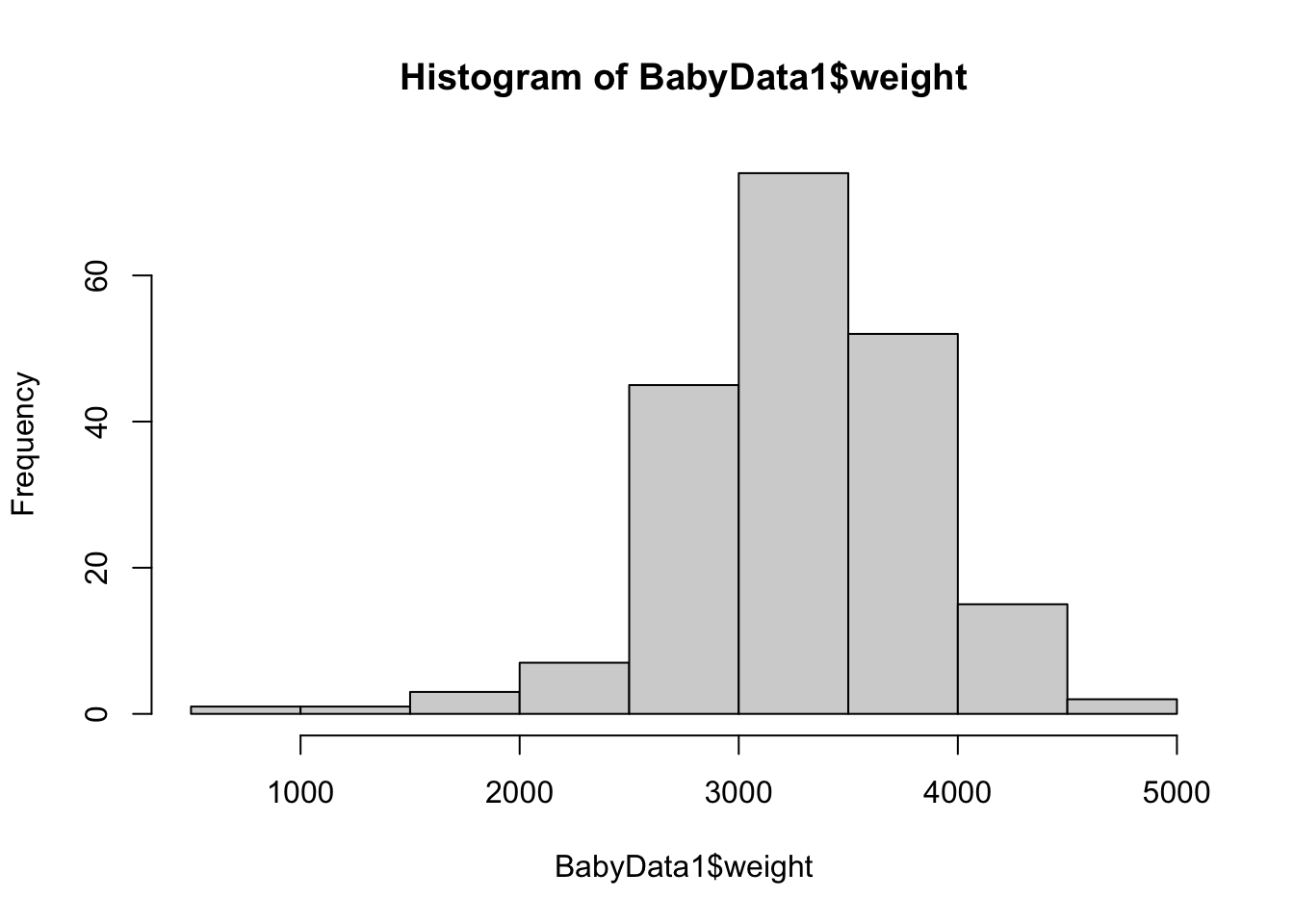
Figure 10.11: Histogram of Babies’ Masses
##    Min. 1st Qu.  Median    Mean 3rd Qu.    Max.
##     907    2935    3325    3283    3629    4825
To make the shift to confidence intervals, we mimic the code we used for sample proportions, but we have changed to using \(t^*\) (or tStar) instead of \(z^*\) (or zStar) and use the appropriate formula for the standard error.
#Data Set
x = BabyData1$weight
#Confidence Level
C.Level = 0.95
#Below here is stock code and should not be changed
x <- x[!is.na(x)]
xBar <- mean(x)            #Sample Mean
s <- sd(x)                 #Sample Standard Deviation
n <- length(x)             #Sample Size
tStar <- qt( 1 - (1 - C.Level) / 2, df = ( n - 1 ) )
SE <- s / sqrt( n )        #Standard Error
MOE <- tStar * SE          #Margin Of Error
CIL <- xBar - MOE          #Confidence Interval Lower Bound
CIU <- xBar + MOE          #Confidence Interval Upper Bound
c( CIL, CIU )              #Confidence Interval
## [1] 3203.396 3361.994This says that we are 95% confident that the population mean of the birth mass of babies is between roughly 3203 and 3362 grams. In terms of weight, this is approximately between 7 pounds 1 ounce and 7 pounds 6.6 ounces.
This does NOT say that 95% of babies will be born with a mass in the above interval. This is only a statement about the population mean.
Using the techniques in Example 10.9, find confidence intervals for the birth mass of male babies at the 95% and 98% confidence levels.
Recall that 95% confidence means that if we were to have 100 samples and produce 100 confidence intervals from those samples, that we would expect 95 of the confidence intervals to correctly capture \(\mu\) and expect 5 samples to be extreme enough to give a confidence interval that does not contain \(\mu\).
The following Code Template can be used to find a confidence interval “by hand.”
#Data Set
x =
#Confidence Level
C.Level =
#Below here is stock code and should not be changed
x <- x[!is.na(x)]
xBar <- mean(x)            #Sample Mean
s <- sd(x)                 #Sample Standard Deviation
n <- length(x)             #Sample Size
tStar <- qt( 1 - (1 - C.Level) / 2, df = ( n - 1 ) )
SE <- s / sqrt( n )        #Standard Error
MOE <- tStar * SE          #Margin Of Error
CIL <- xBar - MOE          #Confidence Interval Lower Bound
CIU <- xBar + MOE          #Confidence Interval Upper Bound
c( CIL, CIU )              #Confidence Interval
Just like in Section 10.2.3, the Code Template for a confidence interval for a population mean saves the values used in the calculation, but it only displays the confidence interval at the end. If you wanted to see the margin of error, for example, you could simply run MOE in your script or console after running the above code.
Find a 99% confidence interval for the mean age of the mother of a newborn baby using BabyData1.
10.3.3 ConfIntFromSample
This section is optional and uses a custom function developed by the Statypi.
In Chapter 9, there was little chance of confusing how a confidence interval related to individuals versus a population. Each individual either had a specified trait or not and thus could be thought of as having a value of 1 or 0 respectively. As such, no individual could have a value of, say, 0.64 and an interval of form \(( 0.5069532, 0.7730468)\) could not contain any individual’s value.
However, now that we are looking at variables that take on (possibly) continuous values, it is possible for an individual to have a value that is very close to the population mean, \(\mu\). As such, it can be confusing as to what a confidence interval means in relation to individuals, values of \(x\), and samples, values of \(\bar{x}\). The function ConfIntFromSample() is meant to give a visual representation to what we have done so far. It will produce a graphical display of the confidence interval superimposed over a histogram which also shows what we will call a Prediction Interval.
Definition 10.5 For a particular proportion on the interval \((0,1)\), a Prediction Interval is an estimate of an interval where we expect that proportion of all individual values of a distribution to fall.
The most typical type of a prediction interval is a middle interval where we capture the middle proportion. There are also lower and upper prediction intervals as well as the analogous versions of confidence intervals for parameters. However, for simplicity, we will assume all confidence and prediction intervals on Statypus are middle intervals.
Statypus Original Function: See Section 10.5.2 for the code to use this function.
The syntax of ConfIntFromSample is
where the arguments are:
x: The data vector we are using for inference.conf.level: The confidence level for the desired confidence interval.
Example 10.10 Consider the dataframe PlatypusData1 which we last saw in Example 10.3 (where you can find the download link as well).
We will look at the Weight variable.181 This variable contains the mass of each platypus. We will focus our view on only male platypuses.
## Warning in ConfIntFromSample(x = PlatypusData1$Weight[PlatypusData1$Sex == :
## Missing values omitted from calculations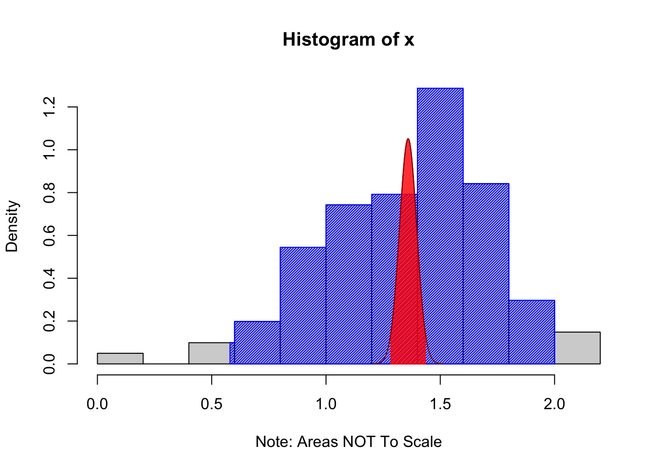
Figure 10.12: Example Using the ConfIntFromSample Function
## $`Confidence Level`
## [1] 0.95
##
## $`Confidence Interval for Mu`
## [1] 1.284502 1.433914
##
## $`Prediction Interval of Individuals`
##  2.5% 97.5%
##  0.58  2.00
The output says that 95% of the values of PlatypusData1$Weight occurred between 0.58 and 2.00 kilograms for males and this would be our best guess for where 95% of all values of male platypuses would fall. The shaded blue region shows the middle 95% of values of our sample laid upon the histogram. This is what is called the Prediction Interval in the code above. The Prediction Interval is our best guess as to where 95% (the confidence level) of individual values will fall.
In contrast, we can say that we are 95% confident that the true population mean of male platypus masses is between 1.284502 and 1.433914 kilograms. The distribution of possible values of \(\bar{x}\) (based on our sample) is shown in dark red and the middle 95% of these values is shown in red. This is what we take as our confidence interval for \(\mu\). If we were to obtain 100 samples and produce 100 confidence intervals, we would expect that 95 out of 100 of them would contain \(\mu\).
The methods used to create the prediction interval here are crude, but meant to show the difference between where we have confidence about individuals as compared to the where we have confidence about the population mean.
We show that the methods given in Section 10.3.2 give the same result below.
#Data Set
x = PlatypusData1$Weight[ PlatypusData1$Sex == "M" ]
#Confidence Level
C.Level = 0.95
#Below here is stock code and should not be changed
x <- x[!is.na(x)]
xBar <- mean(x)            #Sample Mean
s <- sd(x)                 #Sample Standard Deviation
n <- length(x)             #Sample Size
tStar <- qt( 1 - (1 - C.Level) / 2, df = ( n - 1 ) )
SE <- s / sqrt( n )        #Standard Error
MOE <- tStar * SE          #Margin Of Error
CIL <- xBar - MOE          #Confidence Interval Lower Bound
CIU <- xBar + MOE          #Confidence Interval Upper Bound
c( CIL, CIU )              #Confidence Interval
## [1] 1.284502 1.433914Replicate the work in Example 10.10 for
only female platypuses.
only juvenile platypuses.
all platypuses.
10.3.4 t.test to the Rescue Yet Again
In Section 10.2.4, we saw how quickly RStudio handled confidence intervals with just one line of code using t.test. As the output we saw above also displayed a \(p\)-value and we know that binom.test allowed us to do both confidence intervals and hypothesis tests, it is not surprising that we can also use t.test to handle confidence intervals.
Example 10.11 With the help of t.test, we can redo the calculations made in Example 10.9 with one line of code.
##
##  One Sample t-test
##
## data:  BabyData1$weight
## t = 81.632, df = 199, p-value < 2.2e-16
## alternative hypothesis: true mean is not equal to 0
## 95 percent confidence interval:
##  3203.396 3361.994
## sample estimates:
## mean of x
##  3282.695
The output of t.test should be familiar to the reader as it closely mirrors that of binom.test. Moreover, the numerical outputs for the 95% confidence interval match the ones we found in Example 10.9 exactly.
Example 10.12 We will revisit one of our common dataframes here once again, BabyData1. If we simply want a 95% confidence interval for the age of a mother (mom_age), we can use the following simple line of code.
##
##  One Sample t-test
##
## data:  BabyData1$mom_age
## t = 57.984, df = 199, p-value < 2.2e-16
## alternative hypothesis: true mean is not equal to 0
## 95 percent confidence interval:
##  25.68087 27.48913
## sample estimates:
## mean of x
##    26.585
This shows us that we are 95% confident that the true population mean of a woman at the time she gives birth is between approximately 25.681 years and 27.489 years of age. With a point estimate of 26.585 years of age, this gives a margin of error of less than one year.
If we wanted to have a bit more confidence in our estimate, we can increase the value of conf.level, but are reminded that the margin of error will necessarily increase.
##
##  One Sample t-test
##
## data:  BabyData1$mom_age
## t = 57.984, df = 199, p-value < 2.2e-16
## alternative hypothesis: true mean is not equal to 0
## 99 percent confidence interval:
##  25.39257 27.77743
## sample estimates:
## mean of x
##    26.585
Our margin of error for a 99% confidence interval is now almost 1.2 years offering a wider interval which is more likely (99% confidence) to capture the true population mean.
Do the same analysis for the dad_age variable of BabyData1 as done for mom_age in Example 10.12.
Review for Chapter 10 Part 3
Inference for Population Mean(s) Quiz: Part 3
This quiz tests your understanding of Confidence Intervals for a Population Mean (t-Interval). The answers can be found prior to the Exercises section.
- True or False: A confidence interval for the population mean provides a range of plausible values for the true population mean, \(\mu\).
- True or False: The point estimate for the population mean \(\mu\) is the observed sample standard deviation, \(s_x\).
- True or False: The Margin of Error (MOE) for a confidence interval for a population mean is calculated as the critical \(z\)-value (\(z^*\)) multiplied by the Standard Error (SE).
- True or False: The critical value, \(t^*\), is determined by the desired confidence level and the degrees of freedom, which is \(\nu = n-1\).
- True or False: The Standard Error (SE) for the \(t\)-interval uses the sample standard deviation, \(s_{\bf x}\), in its formula: \(\text{SE} = \frac{s_{\bf x}}{\sqrt{n}}\).
- True or False: A prediction interval gives a prediction as to the value of a population parameter.
- True or False: The \(t\)-interval is used instead of a \(z\)-interval because the population mean, \(\mu\), is unknown.
- True or False: The R function
qt()is used to find the critical value \(t^*\) needed to calculate the margin of error. - True or False: Assuming the necessary conditions are met, the R function
t.test()automatically calculates the confidence interval for the population mean. - True or False: A \(95\%\) confidence interval means that \(95\%\) of all random samples will produce an interval that contains the true population mean, \(\mu\).
Definitions
Big Ideas
Section 10.3.2
The best approximation we can make for the Margin Of Error, MOE in R, is
\[z^* \cdot \frac{\sigma_X}{\sqrt{n}} \approx t^* \cdot \frac{s_{\bf x}}{\sqrt{n}}\]
which means that we can rewrite our confidence interval as follows.
\[\text{Point Estimate} \pm \text{Margin Of Error} = \bar{x} \pm z^* \cdot \frac{\sigma_X}{\sqrt{n}} \approx \bar{x} \pm t^* \cdot \frac{s_{\bf x}}{\sqrt{n}}\]
Important Remarks
Section 10.3.2
Recall that 95% confidence means that if we were to have 100 samples and produce 100 confidence intervals from those samples, that we would expect 95 of the confidence intervals to correctly capture \(\mu\) and expect 5 samples to be extreme enough to give a confidence interval that does not contain \(\mu\).
Just like in Section 10.2.3, the Code Template for a confidence interval for a population mean saves the values used in the calculation, but it only displays the confidence interval at the end. If you wanted to see the margin of error, for example, you could simply run MOE in your script or console after running the above code.
Section 10.3.3
The most typical type of a prediction interval is a middle interval where we capture the middle proportion. There are also lower and upper prediction intervals as well as the analogous versions of confidence intervals for parameters. However, for simplicity, we will assume all confidence and prediction intervals on Statypus are middle intervals.
Code Templates
Section 10.3.2
The following Code Template can be used to find a confidence interval “by hand.”
#Data Set
x =
#Confidence Level
C.Level =
#Below here is stock code and should not be changed
x <- x[!is.na(x)]
xBar <- mean(x)            #Sample Mean
s <- sd(x)                 #Sample Standard Deviation
n <- length(x)             #Sample Size
tStar <- qt( 1 - (1 - C.Level) / 2, df = ( n - 1 ) )
SE <- s / sqrt( n )        #Standard Error
MOE <- tStar * SE          #Margin Of Error
CIL <- xBar - MOE          #Confidence Interval Lower Bound
CIU <- xBar + MOE          #Confidence Interval Upper Bound
c( CIL, CIU )              #Confidence Interval
New Functions
Section 10.3.1
The syntax of qt() is
where the arguments are:
p: The probability to be bound by the output.df: Degrees of freedom. It must be positive but may be a non-integer.df = Infis allowed.lower.tail: This option controls whether the quantity returned is an upper or lower bound. Iflower.tail = TRUE(orT), then the output is the quantityqsuch thatP( t \leq q ) = p. Iflower.tailis set toFALSE(orF), then the output is the quantileqsuch thatP( t > q ) = p. If no value is set, R will default tolower.tail = TRUE.
Quiz Answers
- True
- False (The point estimate for the population mean \(\mu\) is the sample mean, \(\bar{x}\).)
- False (The MOE for a \(t\)-interval uses the critical \(t\)-value (\(t^*\)), not the \(z\)-value, as it relies on the \(t\)-distribution.)
- True
- True
- False (A prediction interval is an estimate of an interval where we expect the middle proportion of all individual values of a distribution to fall.)
- False (The \(t\)-interval is used because the population standard deviation, \(\sigma\), is unknown and must be estimated using \(s_{\bf x}\).)
- True
- True
- True
Exercises
Exercise 10.6 According to Snickers.com, as of early 2025, the weight of a Snickers bar in the United States is 1.86 ounces. See Section 6.4 to get the code to load the Snickers dataset into your RStudio environment. Use this dataset to produce a 98% confidence interval for the population mean weight of a Snickers bar. Use both the techniques from Section 10.3.2 and 10.3.4.
Exercise 10.7 In Example 10.10, you used the ConfIntFromSample() function to visualize weight distributions for male platypuses. Now, use the standard t.test() function to find a precise estimate for the whole population.
- Calculate a 99% confidence interval for the population mean
Weight. - Interpret the interval: What does this range tell us about our estimate of the “average” platypus? <!–
##
##  One Sample t-test
##
## data:  PlatypusData1$Weight
## t = 40.822, df = 201, p-value < 2.2e-16
## alternative hypothesis: true mean is not equal to 0
## 99 percent confidence interval:
##  1.053055 1.196351
## sample estimates:
## mean of x
##  1.124703
–>
Exercise 10.8 In Exercise 10.4, we investigated the mercury concentration in Platypuses. Using the mercury concentration data in PlatypusData1, run the ConfIntFromSample() function provided in Section 10.5.2. Based on the plot, explain why a Prediction Interval (showing where an individual platypus might fall) is significantly wider than the Confidence Interval (showing where the population mean is likely located).
10.4 Part 4: Two Sample Population Means
Rather than looking at a single set of data in isolation, we often compare different sets of data. This may be from different columns in the same dataframe, entirely different datasets, or pulling subsets of data based on a certain trait, e.g. selecting 4 cylinder cars out of mtcars. The tools we used to do inference for one sample above can be used to analyze these cases as well and t.test will make quick work of most of our needs.
10.4.1 Hypothesis Tests
The standard setup for hypothesis tests for 2 samples is below.
\[\begin{align*} H_0 &: \mu_1 - \mu_2 = \mu_0\\ H_a &: \mu_1 - \mu_2 \; \Box \; \mu_0 \end{align*}\]
where \(\Box\) can be one of the symbols: \(\neq\), <, or >. RStudio displays the alternative hypothesis by comparing the “true difference in means” to 0 or the value we input as mu. That is, we set \(\mu_0\) to mu and this value is the hypothesized difference between the two population means.
If we set mu to be 0, we can realize the above hypotheses as follows.
\[\begin{align*} H_0 &: \mu_1 = \mu_2\\ H_a &: \mu_1 \; \Box \;\mu_2 \end{align*}\]
This can be done in one of two ways: paired data and non-paired data.
In some experiments, data naturally arises in pairs. That is, we can look at two values, say \(x\) and \(y\), from each individual and either ask if \(x \;\Box\; y\) or equivalently if \(x - y \;\Box\; 0\) (where \(\Box\) can be one of the symbols: \(\neq\), <, or >). The key point of paired data is that both of values \(x\) and \(y\) are explicitly tied to a single individual and not just single values from non-linked vectors \(\bf x\) and \(\bf y\).
Example 10.13 In this chapter, we first encountered the dataset BabyData1 in Example 10.9 where it can also be downloaded. Taken at a very simple biological viewpoint, each newborn has a unique mother and father. The age of these people at the time of the baby’s birth are given by the variables mom_age and dad_age respectively. We can look at each sample as a histogram.
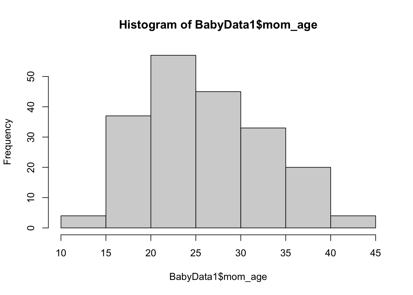
Figure 10.13: Histogram of Ages of Mothers
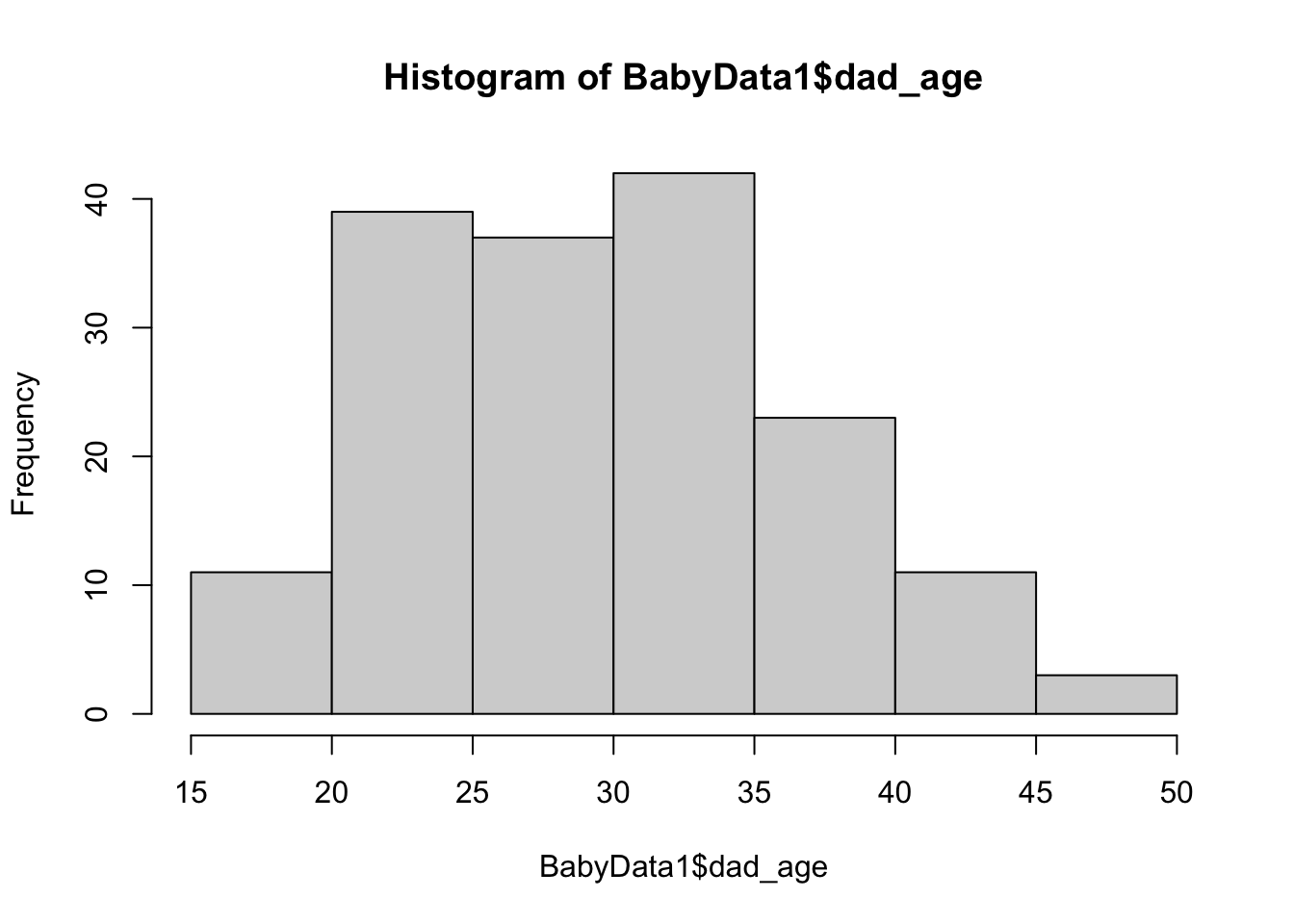
Figure 10.14: Histogram of Ages of Fathers
The histograms seem to encourage the belief that the population mean of the age of a newborn’s mother is less than the population mean age of the newborn’s father. That is, if \(\mu_{\text{diff}}\) is the population mean of the variable of a baby’s mother’s age minus its father’s age (at the time of their birth), we want to run the following hypothesist test.
\[\begin{align*} H_0 &: \mu_{\text{diff}} = 0\\ H_a &: \mu_{\text{diff}} < 0 \end{align*}\]
Since each baby is a single individual, we will begin by simply pulling the individuals where we have both the mother and father’s ages.182
xVec = BabyData1$mom_age
yVec = BabyData1$dad_age
OK <- complete.cases(xVec, yVec)
momAges <- xVec[OK]
dadAges <- yVec[OK]
Now that we have restricted to just the babies that had both mom and dad ages recorded, we can construct a new vector which is the measure of the mom’s age minus the dad’s age. We call this new vector diffAges and run str on it.
## int [1:166] 0 1 -7 -5 -5 -12 -6 2 -2 -5 ...This shows us that diffAges is an integer vector containing 166 entries. For the first baby in our sample, the mom and dad were the same age. The second baby had a mother who was one year older than the dad and the third baby had a mom who was 7 years younger than the dad. The vector diffAges is precisely the type of data we can pass to t.test. We choose alternative = "less" because we predicted that mothers are younger than fathers (on average).
##
##  One Sample t-test
##
## data:  diffAges
## t = -6.82, df = 165, p-value = 8.2e-11
## alternative hypothesis: true mean is less than 0
## 95 percent confidence interval:
##       -Inf -1.879955
## sample estimates:
## mean of x
## -2.481928
This shows that we have sufficient evidence to support the alternative hypothesis that the true mean of the difference momAges - dadAges is less than 0. That is, we have sufficient evidence that a newborn’s mother is younger than their father.
10.4.2 New syntax of t.test
It may not come as a surprise (especially if you have viewed the ?t.test help file), that t.test is quite capable of handling the data vectors mnomAges and dadAges above directly. In fact, the syntax of t.test() we mentioned before left out a couple of arguments, y and paired, which we want to now use as we have more than one data vector. We do this as seen below and remind the reader that we only use conf.level for confidence intervals and save the use of both mu and alternative for hypothesis tests.
While we used t.test before, this gives the new syntax for two sample tests.
#This code will not run unless the necessary values are inputted.
t.test( x, y, conf.level, mu, alternative , paired)
where the arguments are:
x: The first data vector.y: The second data vector.conf.level: The confidence level for the desired confidence interval. Not needed for hypothesis test.mu: The assumed value of \(\mu_X\) in the null hypothesis. Not needed for confidence intervals.muwill default to 0 if not entered.alternative: The symbol in the alternative hypothesis in a hypothesis test. Must be one of"two.sided","less", and"greater". DO NOT USE for confidence intervals.paired: A logical indicating whether you want a paired t-test.
In practice, there is no difference for the user in a paired versus non-paired situation other than selecting the correct value of paired. By default, paired is set to FALSE and if the user tries to use the paired = TRUE method for non-paired data, there is a good chance that RStudio will return an error (unless the two data sets had the same sample size, by chance).
Example 10.14 As a quick example, we can pass momAges and dadAges from Example 10.13 to t.test using this new syntax rather than passing it diffAges (or even momAges - dadAges).
##
##  Paired t-test
##
## data:  momAges and dadAges
## t = -6.82, df = 165, p-value = 8.2e-11
## alternative hypothesis: true mean difference is less than 0
## 95 percent confidence interval:
##       -Inf -1.879955
## sample estimates:
## mean difference
##       -2.481928
This gives the exact same output as we saw in Example 10.13 and thus our conclusion is still the same. In fact, even the degrees of freedom is unchanged at 165 (which is one less than the number of pairs of ages we had).
It is also very useful to mention that t.test will automatically handle the complete.cases situation we handled manually before. We will simply offer up the two columns of t.test and see what happens.
##
##  Paired t-test
##
## data:  BabyData1$mom_age and BabyData1$dad_age
## t = -6.82, df = 165, p-value = 8.2e-11
## alternative hypothesis: true mean difference is less than 0
## 95 percent confidence interval:
##       -Inf -1.879955
## sample estimates:
## mean difference
##       -2.481928
As this code matches our results thus far, we see that t.test can handle this with no need for us to “clean up” the data.
The fact that the outputs of Examples 10.13 and 10.14 are identical gives evidence that the paired version of the two sample test is equivalent to doing a one sample test on the difference of the paired vectors.
We have had a pretty easy path thus far and haven’t needed to even introduce any new statistical or mathematical tools. However, the next example shows that it is too early to get cocky. Thus far, we have assumed that both of our samples come from populations that have identical standard deviations, \(\sigma_1\) and \(\sigma_2\),. The two sample procedures known as Welch’s method performed by t.test(), when we do not set paired = TRUE, do not require the assumption that the two population standard deviations are equal.
Example 10.15 Let’s look at the dataset called candytuft.
Use the following code to download candytuft.
This data originates from the book The Effects of Cross and Self Fertilisation in the Vegetable Kingdom183 by Charles Darwin. There were 30 candytuft plants born from self fertilization and 30 plants born from cross fertilization.
If we let \(x_c\) (or xc in R) be the growth (in inches) of each plant born of cross fertilization and \(x_s\), (or xs) be the growth (in inches) of each plant born of self fertilization, we can do a simple t.test on xc and xs where we set paired = FALSE and choosing to test if \(\mu_c\) (the population mean of cross fertilized candytufts) is greater than \(\mu_s\) (for self fertilized offspring). That is we are testing the following hypotheses.
\[\begin{align*} H_0 &: \mu_c = \mu_s\\ H_a &: \mu_c > \mu_s \end{align*}\]
xc = candytuft$cross
xs = candytuft$self
t.test( x = xc, y = xs, paired = FALSE,
        alternative = "greater" )
##
## Welch Two Sample t-test
##
## data: xc and xs
## t = 3.4524, df = 48.436, p-value = 0.0005814
## alternative hypothesis: true difference in means is greater than 0
## 95 percent confidence interval:
## 1.208541 Inf
## sample estimates:
## mean of x mean of y
## 17.34583 14.99583A \(t\)-statistic of 3.4524 seems normal and we also have a nice low \(p\)-value. However, sitting right between these values is the statement
df = 48.436
which may bewilder people at first. Up until this point, the degrees of freedom argument has always been one less than the sample size, but now we are getting decimal points in our df value!
The above example shows that the concept of degrees of freedom can be more subtle than just the \({n-1}\) that we have seen thus far. This means we need some way of finding the degrees of freedom that occurs when we analyze two non-paired datasets.
Theorem 10.1 For non-paired data, the test statistic for a two sample population mean hypothesis test is given by \[t = \frac{(\bar{x}_1 - \bar{x}_2) - \mu_0}{\sqrt{\frac{s_1^2}{n_1} + \frac{s_2^2}{n_2}}}\] with the degrees of freedom given by \[df = \frac{\left(\frac{s_1^2}{n_1} + \frac{s_2^2}{n_2}\right)^2} {\frac{\frac{s_1^2}{n_1}}{n_1 -1} + \frac{\frac{s_2^2}{n_2}}{n_2-1}}\] where \(s_k\) and \(n_k\) are the sample standard deviation and sample size of sample \(k\) respectively.
We remind the reader that we are assuming that \(\mu_1 - \mu_2\) is the value given in \(H_0\), namely \(\mu_0\) or mu within t.test.
Confirm that the \(t\)-statistic as well as the value of df found in Example 10.15 above match with the theoretical values given in Theorem 10.1. We won’t do this again, but checking it once is always good for our own confidence.
Example 10.16 (Fuel Efficiencies) We want to test whether the population mean of fuel efficiency of 4 cylinder cars was at least 5 mpg greater than that of 6 cylinder cars. To this aim, we set \(\mu_1\) to be the population mean of fuel efficiency of 4 cylinder cars and set \(\mu_2\) to be the population mean of fuel efficiency of 6 cylinder cars. The hypotheses we have are as follows.
\[\begin{align*} H_0 &: \mu_1 - \mu_2 = 5\\ H_a &: \mu_1 - \mu_2 > 5 \end{align*}\]
We will need data to test now. Using the mtcars dataframe, we know that mtcars$mpg gives us the measure of fuel efficiency, but this would be for all cars in the sample. We need to separate off the 4 cylinder and 6 cylinder cars.
We can do this by setting \(x\) to be mtcars$mpg[ mtcars$cyl==4 ] which takes the subset of the vector, mtcars$mpg, where the value in the cyl column is 4. We analogously set \(y\) to be mtcars$mpg[ mtcars$cyl==6 ]. The only other argument we must input into t.test is the alternative and as our alternative contains the symbol “>”, we set alternative to be "greater". We also set mu to be 5 for the assumed disparity between \(\mu_1\) and \(\mu_2\).
t.test( x = mtcars$mpg[ mtcars$cyl==4 ],
        y = mtcars$mpg[ mtcars$cyl==6 ],
        mu = 5, alternative = "greater" )
##
## Welch Two Sample t-test
##
## data: mtcars$mpg[mtcars$cyl == 4] and mtcars$mpg[mtcars$cyl == 6]
## t = 1.3097, df = 12.956, p-value = 0.1065
## alternative hypothesis: true difference in means is greater than 5
## 95 percent confidence interval:
## 4.322926 Inf
## sample estimates:
## mean of x mean of y
## 26.66364 19.74286This gives a \(p\)-value of over 10% which will be greater than any \(\alpha\) worth considering. There is over a 10% chance that \(H_0\) is true and we would still see data like this by chance. That is, we have insufficient evidence to reject \(H_0\), or that 4 cylinder cars have a fuel efficiency (no more than) 5 mpg greater than that of 6 cylinder cars on average.
Example 10.17 We begin by loading the TitanicDataset with the following command.
Use the following code to download TitanicDataset.
The dictionary for the dataset can be found here. We begin by looking at it with str.
## 'data.frame':    891 obs. of  11 variables:
##  $ Survived: int  0 1 1 1 0 0 0 0 1 1 ...
##  $ Pclass  : int  3 1 3 1 3 3 1 3 3 2 ...
##  $ Name    : chr  "Braund, Mr. Owen Harris" "Cumings, Mrs. John Bradley (Florence Briggs Thayer)" "Heikkinen, Miss. Laina" "Futrelle, Mrs. Jacques Heath (Lily May Peel)" ...
##  $ Sex     : chr  "male" "female" "female" "female" ...
##  $ Age     : num  22 38 26 35 35 NA 54 2 27 14 ...
##  $ SibSp   : int  1 1 0 1 0 0 0 3 0 1 ...
##  $ Parch   : int  0 0 0 0 0 0 0 1 2 0 ...
##  $ Ticket  : chr  "A/5 21171" "PC 17599" "STON/O2. 3101282" "113803" ...
##  $ Fare    : num  7.25 71.28 7.92 53.1 8.05 ...
##  $ Cabin   : chr  "" "C85" "" "C123" ...
##  $ Embarked: chr  "S" "C" "S" "S" ...
You may have heard the saying “Women and Children First” about who to prioritize saving during a disaster. Does this mean we should expect the average age of a survivor is less than that of the group of individuals who perished?
That is, if we let \(\mu_S\) be the mean age of Titanic passengers who Survived and \(\mu_P\) be the mean age of those passengers who Perished, we wish to test the following hypotheses.
\[\begin{align*} H_0 &: \mu_S = \mu_P\\ H_a &: \mu_S < \mu_P \end{align*}\]
We can do this easily with t.test. To streamline our code, we will create a copy of TitanicDataset called df (short for dataframe).
df <- TitanicDataset
t.test( x = df$Age[ df$Survived == 1 ],
        y = df$Age[ df$Survived == 0 ],
        alternative = "less" )
##
## Welch Two Sample t-test
##
## data: df$Age[df$Survived == 1] and df$Age[df$Survived == 0]
## t = -2.046, df = 598.84, p-value = 0.02059
## alternative hypothesis: true difference in means is less than 0
## 95 percent confidence interval:
## -Inf -0.4446974
## sample estimates:
## mean of x mean of y
## 28.34369 30.62618Our \(p\)-value falls in that awkward region between 0.01 and 0.05. Our evidence is sufficient if we only lower \(\alpha\) to 0.05, but if we lower \(\alpha\) to 0.01, then our evidence fails to be sufficient at this stricter level of significance.
The verdict of this hypothesis test truly depends on the level of evidence that the user demands.
Example 10.18 (Does Gender Affect Birth Weight?) We can return to the dataframe BabyData1 we used earlier to investigate the question of whether birth weight depends on the gender of the baby. That is, is the population mean birth weight for male babies different than that of the population mean birth weight of female babies. If we let \(\mu_M\) be the population mean birth weight of male babies and \(\mu_F\) be the population mean birth weight of female babies, we want to conduct the following hypothesis test.
\[\begin{align*} H_0 &: \mu_M = \mu_F\\ H_a &: \mu_M \neq \mu_F \end{align*}\]
Being that this is a two tailed test with \(\mu_0 = 0\), we can simply run the following code where we use dd (like we used the more descriptive df previously) here as a copy of BabyData1.
##
##  Welch Two Sample t-test
##
## data:  dd$weight[dd$sex == "M"] and dd$weight[dd$sex == "F"]
## t = 0.4348, df = 197.8, p-value = 0.6642
## alternative hypothesis: true difference in means is not equal to 0
## 95 percent confidence interval:
##  -123.5984  193.5179
## sample estimates:
## mean of x mean of y
##  3299.650  3264.691
Recall that before we ran the test, our “belief” in \(H_0\) was 100% or 1.00. However, after running the test, we now only have a 66.42% belief in \(H_0\). This is obviously way higher than most of the \(p\)-values we normally encounter and it is clear we have very poor evidence for \(H_a\). At any reasonable \(\alpha\) level, we would be unable to reject \(H_0\). That is, there is not sufficient evidence that \(\mu_M \neq \mu_F\).
If you are curious why we used dd here, try redoing Example 10.18 without this “trick” and type out BabyData1 whenever necessary.
10.4.3 Confidence Intervals
Before, we were looking for a confidence interval that captured \(\mu\). Now, we are looking for a confidence interval that captures the difference of two population means. If \(\mu_1\) and \(\mu_2\) are our population means, we are looking for a confidence interval for \(\mu_1 - \mu_2\). When comparing two independent or non-paired means, the point estimate for the difference \(\mu_1 - \mu_2\) is the difference in the sample means, \(\bar{x}_1 - \bar{x}_2\).
In practice, there is no difference for the user in a paired versus non-paired situation other than selecting the correct value of paired.
If you simply input
t.test( x, y )you will get a 95% confidence interval for \(\mu_1 - \mu_2\) and a hypothesis test testing if \(\mu_1 - \mu_2 \neq 0\).We can still invoke the
pairedargument when we have paired data.
Example 10.19 We return to TitanicDataset which we downloaded in Example 10.17. In that example, it appeared that survivors were over 2 years younger (on average) than those who perished. We can now use t.test to get a confidence interval for the difference in the mean ages of the two groups where we once again use the df “copy” of TitanicDataset to streamline our code.
##
##  Welch Two Sample t-test
##
## data:  df$Age[df$Survived == 1] and df$Age[df$Survived == 0]
## t = -2.046, df = 598.84, p-value = 0.04119
## alternative hypothesis: true difference in means is not equal to 0
## 95 percent confidence interval:
##  -4.47339446 -0.09158472
## sample estimates:
## mean of x mean of y
##  28.34369  30.62618
This gives a confidence interval of \((-4.47339446, -0.09158472)\) which means that we are 95% confident that the difference in means may be as little as around a tenth of a year but may be as much as nearly 4.5 years.
We could have included the argument conf.level = 0.95, but t.test will default to this value. This is helpful to remember when you simply want to run a quick test to quickly look at your data.
Find a 99% confidence interval for the difference in concentration levels of male versus female platypuses using the PlatypusData1 dataset.
Review for Chapter 10 Part 4
Inference for Population Mean(s) Quiz: Part 4
This quiz tests your understanding of Inference for the Difference of Two Independent Population Means. The answers can be found prior to the Exercises section.
- True or False:
Results
Section 10.4.2
Theorem 10.1 \(\;\) For non-paired data, the test statistic for a two sample population mean hypothesis test is given by \[t = \frac{(\bar{x}_1 - \bar{x}_2) - \mu_0}{\sqrt{\frac{s_1^2}{n_1} + \frac{s_2^2}{n_2}}}\] with the degrees of freedom given by \[df = \frac{\left(\frac{s_1^2}{n_1} + \frac{s_2^2}{n_2}\right)^2} {\frac{\frac{s_1^2}{n_1}}{n_1 -1} + \frac{\frac{s_2^2}{n_2}}{n_2-1}}\] where \(s_k\) and \(n_K\) are the sample standard deviation and sample size of sample \(k\) respectively.
Big Ideas
Section 10.4.1
The standard setup for hypothesis tests for 2 samples is below.
\[\begin{align*} H_0 &: \mu_1 - \mu_2 = \mu_0\\ H_a &: \mu_1 - \mu_2 \; \Box \; \mu_0 \end{align*}\]
where \(\Box\) can be one of the symbols: \(\neq\), <, or >. RStudio displays the alternative hypothesis by comparing the “true difference in means” to 0 or the value we input as mu. That is, we set \(\mu_0\) to mu and this value is the hypothesized difference between the two population means.
Important Remarks
Section 10.4.3
If you simply input
t.test( x, y )you will get a 95% confidence interval for \(\mu_1 - \mu_2\) and a hypothesis test testing if \(\mu_1 - \mu_2 \neq 0\).We can still invoke the
pairedargument when we have paired data.
New Functions
Section 10.4.2
While we used t.test before, this gives the new syntax for two sample tests.
#This code will not run unless the necessary values are inputted.
t.test( x, y, conf.level, mu, alternative , paired)
where the arguments are:
x: The first data vector.y: The second data vector.conf.level: The confidence level for the desired confidence interval. Not needed for hypothesis test.mu: The assumed value of \(\mu_X\) in the null hypothesis. Not needed for confidence intervals.muwill default to 0 if not entered.alternative: The symbol in the alternative hypothesis in a hypothesis test. Must be one of"two.sided","less", and"greater". DO NOT USE for confidence intervals.paired: A logical indicating whether you want a paired t-test.
Exercises
For Exercises 10.9 through 10.10, you will need to load the dataset TitanicDataset. The code for this can be found in Example 10.17.
Exercise 10.9 Use a t.test to test if the mean age of males on the Titanic differed from the mean age of females on the Titanic. Specify what test you are running along with the hypotheses and give a conclusion at the \(\alpha = 0.01\) level of significance.
Exercise 10.10 When a ship goes down, is it “Women and Children First” or should we just follow the money? Use a t.test to test if the people who survived the Titanic disaster paid more on average than the people who perished. Specify what test you are running along with the hypotheses and give a conclusion at the \(\alpha = 0.001\) level of significance.
10.5 Appendix
10.5.1 Simulations Verifying Confidence Intervals
Example 10.20 In this example, we run a simulation to see if 95% of samples do give confidence intervals that capture \(\mu\). We will use the distribution of US adult female heights, namely \(\mu=64.5\) and \(\sigma = 2.5\). We will look at samples of size \(n = 25\). We will follow the 4 Step procedure laid out in Chapter 13.
Step 1: Write repeatable code that performs the experiment a single time.
The code below sets up the values which will not change within each iteration of the replicate. We will run it separate and store the values in our environment to streamline our code.
n <- 25
mu <- 64.5
sigma <- 2.5
C.Level <- 0.95    #Confidence Level
tStar = qt( 1 - (1 - C.Level) / 2, df = ( n - 1 ) )
If you want to try this code with different values, you can simply change the values above and rerun the block of code. We now use rnorm to generate a random set of values that satisfy the now set values of \(\mu=64.5\) and \(\sigma = 2.5\). We then carry out the work done in Section #ref(OneSamplePopMeansConfInt) to see if the value of \(\mu\) is in the confidence interval. Note that the code is slightly “slimmer” than the code we used in Section 10.3.1 to allow us to run a very large number of experiments in just a minute.
x <- rnorm( n, mean = mu, sd = sigma )  #Random Data Set
#Below checks if mu is in the Conf. Int.
( ( mu > mean(x) - tStar * sd(x) / sqrt( n ) )
  & ( mu < mean(x) + tStar * sd(x) / sqrt( n ) ) )
## [1] TRUEStep 2: Replicate the experiment a small number of times and check the results.
Now that we believe we have repeatable code, we run a small simulation (100 times should suffice) to make sure that the code is not always either TRUE or FALSE.
replicate(100, {
  x <- rnorm( n, mean = mu, sd = sigma )  #Random Data Set
  #Below checks if mu is in the Conf. Int.
  ( ( mu > mean(x) - tStar * sd(x) / sqrt( n ) )
    & ( mu < mean(x) + tStar * sd(x) / sqrt( n ) ) )
})
## [1] TRUE TRUE TRUE TRUE TRUE TRUE TRUE TRUE TRUE TRUE TRUE TRUE
## [13] TRUE TRUE TRUE TRUE TRUE TRUE TRUE TRUE TRUE TRUE TRUE TRUE
## [25] TRUE TRUE TRUE TRUE TRUE TRUE TRUE FALSE TRUE TRUE TRUE TRUE
## [37] TRUE TRUE TRUE TRUE TRUE TRUE TRUE TRUE TRUE TRUE TRUE TRUE
## [49] FALSE TRUE TRUE TRUE TRUE TRUE TRUE TRUE TRUE FALSE TRUE TRUE
## [61] TRUE TRUE TRUE TRUE TRUE TRUE TRUE TRUE TRUE TRUE TRUE TRUE
## [73] TRUE TRUE TRUE TRUE TRUE FALSE FALSE TRUE TRUE FALSE TRUE TRUE
## [85] TRUE TRUE TRUE TRUE TRUE TRUE TRUE TRUE TRUE TRUE TRUE FALSE
## [97] TRUE TRUE TRUE TRUEThis small simulation shows that 96 out of 100 samples generated created a confidence interval that successfully captured the population proportion. This aligns closely with the 95% Confidence Level we set in Step 1.
Step 3: Replicate the experiment a large number of times and store the result.
We now ramp up the number of samples we test to one million to make sure that our result from Step 2 was accurate.
eventCI <- replicate(1000000, {
  x <- rnorm( n, mean = mu, sd = sigma )  #Random Data Set
  #Below checks if mu is in the Conf. Int.
  ( ( mu > mean(x) - tStar * sd(x) / sqrt( n ) )
    & ( mu < mean(x) + tStar * sd(x) / sqrt( n ) ) )
})
Step 4: Finally, estimate the probability using mean.
We now are able to find the proportion of the one million samples that successfully captured the population mean which we use as the estimate of the probability that a random sample will do the same thing.
## [1] 0.949712This shows that about 94.97% of samples result in confidence intervals that do capture the population mean which is very close to the specified 95% Confidence Level.
Example 10.21 In this example, we run another simulation to see if t.test will give better results than the manual techniques developed in Section 10.3.1. We will again use the distribution of US adult female heights (\(\mu=64.5\) and \(\sigma = 2.5\)) and look at samples of size \(n = 25\). We will follow the 4 Step procedure laid out in Chapter 13.
Step 1: Write repeatable code that performs the experiment a single time.
Like before, we set up the values which will not change within each iteration of the replicate and store the values in our environment to streamline our code.
n <- 25
mu <- 64.5
sigma <- 2.5
C.Level <- 0.95    #Confidence Level
tStar = qt( 1 - (1 - C.Level) / 2, df = ( n - 1 ) )
Once again, you can simply change the values above and rerun the block of code if you want to change the arguments of the simulation. We now use rnorm to generate a set of random values and pass that result into t.test. We first save the result as results and then look at the results.
x <- rnorm( n, mean = mu, sd = sigma )  #Random Data Set
#Below checks if mu is in the Conf. Int.
results <- t.test( x, conf.level = C.Level )
results
##
## One Sample t-test
##
## data: x
## t = 127.09, df = 24, p-value < 2.2e-16
## alternative hypothesis: true mean is not equal to 0
## 95 percent confidence interval:
## 62.55231 64.61745
## sample estimates:
## mean of x
## 63.58488This sample had \(\bar{x}_0 = 63.58488\) and a confidence interval of \((62.55231, 64.61745)\). Thus, it did capture \(\mu\). To test this in a more repeatable way, we can use the values stored in results$conf.int.
## [1] 62.55231 64.61745
## attr(,"conf.level")
## [1] 0.95
We can get at the individual bounds of the confidence interval using results$conf.int[1] and results$conf.int[2]. To expedite our process, we have removed any superfluous code.
results <- t.test( x = rnorm( n, mean = mu, sd = sigma ),
                   conf.level = C.Level )
( mu > results$conf.int[1] ) & ( mu < results$conf.int[2] )
## [1] TRUEStep 2: Replicate the experiment a small number of times and check the results.
Now that we believe we have repeatable code, we run a small simulation (100 times is still good enough) to make sure that the code is not always either TRUE or FALSE.
replicate(100, {
  results <- t.test( x = rnorm( n, mean = mu, sd = sigma ),
                   conf.level = C.Level )
  ( mu > results$conf.int[1] ) & ( mu < results$conf.int[2] )
})
## [1] TRUE TRUE TRUE TRUE TRUE TRUE TRUE TRUE TRUE TRUE TRUE TRUE
## [13] TRUE TRUE TRUE TRUE TRUE TRUE TRUE TRUE TRUE TRUE TRUE TRUE
## [25] TRUE TRUE TRUE TRUE TRUE TRUE TRUE FALSE TRUE TRUE TRUE TRUE
## [37] TRUE TRUE TRUE TRUE TRUE TRUE TRUE TRUE TRUE TRUE TRUE TRUE
## [49] FALSE TRUE TRUE TRUE TRUE TRUE TRUE TRUE TRUE FALSE TRUE TRUE
## [61] TRUE TRUE TRUE TRUE TRUE TRUE TRUE TRUE TRUE TRUE TRUE TRUE
## [73] TRUE TRUE TRUE TRUE TRUE FALSE FALSE TRUE TRUE FALSE TRUE TRUE
## [85] TRUE TRUE TRUE TRUE TRUE TRUE TRUE TRUE TRUE TRUE TRUE FALSE
## [97] TRUE TRUE TRUE TRUEThis small simulation shows that 93 out of 100 samples generated created a confidence interval that successfully captured the population proportion. This is lower than the 95% Confidence Level we set in Step 1, so we will see what happens when we do a large number of samples.
Step 3: Replicate the experiment a large number of times and store the result.
We now ramp up the number of samples we test to one hundred thousand (one million takes a bit too long on most machines) to see how our simulation compares to the set value of C.Level.
eventCIttest <- replicate(100000, {
  results <- t.test( x = rnorm( n, mean = mu, sd = sigma ),
                   conf.level = C.Level )
  ( mu > results$conf.int[1] ) & ( mu < results$conf.int[2] )
})
Step 4: Finally, estimate the probability using mean.
We now are able to find the proportion of the one hundred thousand samples that successfully captured the population mean which we use as the estimate of the probability that a random sample will do the same thing.
## [1] 0.95017This shows that approximately 94.98% of samples result in confidence intervals that do capture the population mean. This means that t.test gives confidence interval that are successful as often as the prescribed confidence level.
10.5.2 ConfIntFromSample Code
Description
ConfIntFromSample generates a confidence interval for the population mean, \(\mu\), as well as a crude prediction interval of the variable.
Usage
ConfIntFromSample( x, conf.level = 0.95 )
Arguments
x a numeric vectors.
conf.level a numeric value on the interval \((0,1)\).
Details
x must be a numeric vector. If not, an Error will be returned.
A histogram is plotted and the shaded blue region shows the middle values of our sample laid upon the histogram playing the role of a prediction interval. The distribution of possible values of \(\bar{x}\) based on our sample is shown in dark red and the middle values are shown in red. The value of conf.level dictates how much of the middle of the distribution is shaded in each case with a value of 95% used as default if no value is provided by the user.
Value
A list containing the following components:
Confidence Level The user chosen confidence level.
Confidence Interval for Mu The confidence interval for \(\mu\).
Prediction Interval of Individuals The prediction interval for \(x\).
Source
Developed by Dr. Phil Huling from Saint Louis University for use in r.statypus.org (2025).
References
Contact Dr. Phil Huling at phil.huling@slu.edu with further questions.
See Also
See r.statypus.org for other functions developed for use in an introductory statistics course..
Examples
# From r.statypus.org Chapter 10
PlatypusData1 <- read.csv( "https://statypus.org/files/PlatypusData1.csv" )
ConfIntFromSample( x = PlatypusData1$Weight[ PlatypusData1$Sex == "M" ] )
Installation Code
Use the following code to install ConfIntFromSample on your machine.
ConfIntFromSample <- function( x, conf.level = 0.95){
  if( !is.numeric( x ) ){
    stop("'x' must be a numeric vector. Consider using `as.numeric`.")
      }
  if( length(x[is.na(x)] != 0)  )
    warning("Missing values omitted from calculations")
  x <- x[!is.na(x)]
  CILp <- (1 - conf.level) / 2
  CIUp <- 1 - CILp
  xBar = mean(x)
  s = sd(x)
  n = length(x)
  tStar = qt( CIUp, df = ( n - 1 ) )
  SE = s / sqrt( n )
  MOE = tStar * SE
  CIL2 = xBar - MOE           #Confidence Interval Lower Bound
  CIU2 = xBar + MOE           #Confidence Interval Upper Bound

  xHist <- hist( x, plot = F )

  xDelta <- xHist$breaks[2] - xHist$breaks[1]
  CIL <- quantile( x, probs = CILp )
  xL <- xHist$breaks[ min(which( xHist$breaks > CIL)) ]
  yL <- xHist$counts[ min(which( xHist$breaks > CIL)) ]

  CIU <- quantile( x, probs = CIUp )
  xR <- xHist$breaks[ max(which( xHist$breaks < CIU)) ]
  yR <- xHist$counts[ max(which( xHist$breaks < CIU)) ]

  CILength <- round((xR - xL) / xDelta)

  xValues <- c( rep(
    c( CIL ,seq( from = xL, to = xR, by = xDelta ),
       CIU ),
    each = 2)
      )
  yValues <- c( 0,
                rep(
                  xHist$density[ min(which( xHist$breaks > CIL)) -2 + 1:(CILength+2)],
                  each = 2),
                0)

  xValues2 <- seq( from = CIL2, to = CIU2, length.out = 100 )
  yValues2 <- dt( x = (xValues2-xBar)/(s/sqrt(n)), df = n-1 )/s

  xValues3 <- seq( from = xBar - 4*SE, to = xBar + 4*SE, length.out = 1000 )
  yValues3 <- dt( x = (xValues3-xBar)/(s/sqrt(n)), df = n-1 )/s

  hist( x, freq = F, ylim = c(0,max(c(yValues3,xHist$density))),
        xlab = "Note: Areas NOT To Scale")
  polygon(xValues,yValues,col='blue', density = 50)
  polygon(c(CIL2, xValues2, CIU2), c(0,yValues2,0),col='red', density = 80)
  lines( xValues3, yValues3, col = "darkred")

  Results <- list("Confidence Level" = conf.level,
                "Confidence Interval for Mu" = c( CIL2, CIU2 ),
                "Prediction Interval of Individuals" = c(CIL, CIU))
  return(Results)
}
10.5.3 tsum.test for Summarized Data
There is a tendency for introductory textbooks to calculate confidence intervals and perform hypothesis testing using only numerical summaries of a dataset. If you go back and look at the constructions we did, we really only needed to know the sample mean, sample standard deviation, and sample size to perform most of the calculations we have done so far.184 As such, a lot of textbooks will simply report these numerical summaries of datasets rather than offering the entire raw dataset. One benefit is immediate, numerical summaries can be reported on a single row of text while complete datasets can span a half of a page (or more). It is clear that publishers do not want to allocate pages of their books to simply displaying datasets. In fact, real datasets are often too large to be properly printed in a textbook regardless.
tsum.test(): Performs a one-sample or two-sample t-test based on user supplied summary information. Output is identical to that produced witht.test.
[Requires theBSDApackage.]
There is no built in function to R that will allow the calculations we have conducted thus far to be made with only numerical summaries of a dataset. Fortunately, the R Package called “BSDA” which stands for “Basic Statistics and Data Analysis” offers just such a function.
You can load this package by running the following code which was introduced in Section 1.3.5:
and then this code:
This package was originally developed for a textbook of the same name. This book has been out of print for many years, but this package is still being maintained by Alan T. Arnholt of The Appalachian State University as of January 2025. The package offers functions which will allow us to run tests with R when we are only given numerical summaries of a dataset as compared to the raw data.
While R has no issue handling all of the computations needed for the course, R is primarily meant to work with raw data and not just with numerical summaries. This nice package helps bridge that gap.
This package is only necessary for the material in section 10.5.3.
The package BSDA offers us the new function tsum.test() which makes the exact same calculations as that of t.test, but it only requires the numerical summaries of the data. The sum in tsum.test can be viewed as the fact that it is t.test but only using summaries of the data, i.e. t-summary test.
The syntax of tsum.test() for one sample confidence intervals and hypothesis testing is
#This code will not run unless the necessary values are inputted.
tsum.test( mean.x, s.x, n.x, conf.level, mu, alternative )
where the arguments are:
mean.x: The mean of the sample data.s.x: The sample standard deviation of the sample.n.x: The sample size of the data.conf.level: The confidence level for the desired confidence interval. Not needed for hypothesis test.mu: The assumed value of \(\mu_X\) in the null hypothesis. Not needed for confidence intervals.alternative: The symbol in the alternative hypothesis in a hypothesis test. Must be one of"two.sided","less", and"greater". DO NOT USE for confidence intervals.
Example 10.22 We can revisit Examples 10.9 and 10.11 and replicate the work with tsum.test. To remind the reader, in Example 10.9 we constructed a confidence for birth mass (let’s not get into that again) based on the BabyData1 data frame. In Example 10.11, we replicated this work using the t.test function and got the output shown below.
##
##  One Sample t-test
##
## data:  data
## t = 81.632, df = 199, p-value < 2.2e-16
## alternative hypothesis: true mean is not equal to 0
## 95 percent confidence interval:
##  3203.396 3361.994
## sample estimates:
## mean of x
##  3282.695
This result exactly matched the confidence interval found in Example 10.9 and if we review that example, we can see that the code first calculated the sample mean, sample standard deviation, and the sample size and then used only those values to calculate the confidence interval. Thus, R does not need the raw data in order to calculate a confidence interval and thus we have some faith that tsum.test will be successful. This is indeed the case as shown below.
## Warning in tsum.test(mean.x = mean(data), s.x = sd(data), n.x = length(data)):
## argument 'var.equal' ignored for one-sample test.
##
## One-sample t-Test
##
## data: Summarized x
## t = 81.632, df = 199, p-value < 2.2e-16
## alternative hypothesis: true mean is not equal to 0
## 95 percent confidence interval:
## 3203.396 3361.994
## sample estimates:
## mean of x
## 3282.695This shows us that the output of tsum.test is identical to that output of t.test.
The function tsum.test will always throw a warning about the var.equal argument when conducting a one sample test. This argument only has an application for two sample tests and the warning can be overlooked.
To handle two sample inferences, we just need to pass more arguments to tsum.test.
The syntax of tsum.test() for two sample confidence intervals and hypothesis testing is
#This code will not run unless the necessary values are inputted.
tsum.test( mean.x, s.x, n.x, mean.y, s.y, n.y, conf.level, mu, alternative )
where the new arguments are:
mean.y: The mean of the second sample.s.y: The sample standard deviation of the second sample.n.y: The sample size of the second sample.
Example 10.23 With our new syntax for tsum.test, we can revisit the hypothesis test conducted in Example 10.15, where you can download the dataset if needed. In that example, we tested if the average growth of plants born from cross fertilization was greater than those born from self fertilization. That is, we wanted to run the following hypothesis test.
\[\begin{align*} H_0 &: \mu_c = \mu_s\\ H_a &: \mu_c > \mu_s \end{align*}\]
Once difference from Example 10.15 is that we change the notation from xc and xs (to signify “cross” and “self” respectively) to x and y (to match the syntax of tsum.test).
x = candytuft$cross
y = candytuft$self
tsum.test( mean.x = mean(x), s.x = sd(x), n.x = length(x),
           mean.y = mean(y), s.y = sd(y), n.y = length(y),
           alternative = "greater")
##
## Welch Modified Two-Sample t-Test
##
## data: Summarized x and y
## t = 3.4524, df = 48.436, p-value = 0.0005814
## alternative hypothesis: true difference in means is greater than 0
## 95 percent confidence interval:
## 1.208541 NA
## sample estimates:
## mean of x mean of y
## 17.34583 14.99583The function tsum.test will display two sample tests as “Welch Modified Two-Sample t-Test,” but the calculations match that of “Welch Two-Sample t-Test” found in t.test. This distinction should not affect any calculations made.
As mentioned in a footnote earlier, tsum.test cannot be used for paired data as we need more than just the summaries of the two data vectors to run this test. The issue is that sd( x - y ) cannot be calculated from sd( x ) and sd( y ) without knowing if x and y are independent or not.
Fauna of Australia. Vol. 1b. Australian Biological Resources Study (ABRS)↩︎
Like before, it is important to know that the technical meaning of the \(p\)-value is much more nuanced. However, this basic mentality can make it much easier to understand the logic behind hypothesis tests.↩︎
Student was a pseudonym of William Gosset used in order to publish his work while working at the Guiness Brewery in Dublin, Ireland. His work revolutionized the accuracy of small sample inferences about a population mean.↩︎
The formula for Student’s \(t\)-distribution is beyond the scope of this document as it requires a good amount of calculus.↩︎
See Wikipedia if you want to investigate the concept of heavy tailed distributions further.↩︎
While not obvious why, we will also want to consider degrees of freedom which are not natural numbers. This will allow us to give more precise results when we transition to inferences about two samples. This is why there is a toggle for Discrete versus Continuous on the visualization linked below. This also explains why a lot of sources use \(\nu\) for the degrees of freedom in lieu of \(n\), which is often reserved for integers.↩︎
Formally, if we let \(t_\nu\) be Student’s \(t\)-Distribution with \(\nu\) degrees of freedom, then \[\lim_{\nu \rightarrow \infty} t_\nu = \text{Norm}(0,1).\]↩︎
Yes, the way it is displayed here is actually 2 lines of code, but it is only a single function call and could be shown on a single line. The Statypi have chosen to break it up this way so that it is easier to read on your screen.↩︎
We have beaten this proverbial horse to death at this point, but as a reminder, we are conflating mass and weight here.↩︎
The formula for Student’s \(t\)-distribution is beyond the scope of this document as it requires a good amount of calculus.↩︎
While not obvious why, we will also want to consider degrees of freedom which are not natural numbers. This will allow us to give more precise results when we transition to inferences about two samples. This is why there is a toggle for Discrete versus Continuous on the visualization linked below. This also explains why a lot of sources use \(\nu\) for the degrees of freedom in lieu of \(n\), which is often reserved for integers.↩︎
See Wikipedia if you want to investigate the concept of heavy tailed distributions further.↩︎
Insert your own joke here for this cutie.↩︎
This is getting tiresome to point out at this point, but this is technically a measure of mass and not weight as it is labeled. For a deeper dive, see the footnote in Example 5.8 in Section 5.4.↩︎
We do not go into much detail about the
complete.cases()function here at Statypus. Feel free to see?complete.casesif you want to dig a bit deeper.↩︎This book, although written in 1876, is still cited as a work discussing the dangers of inbred populations.↩︎
tsum.testcannot be used for paired data as we need more than just the summaries of the two data vectors to run this test. The issue is thatsd( x - y )cannot be calculated fromsd( x )andsd( y )without knowing ifxandyare independent or not.↩︎