Chapter 1 Introduction to R

Figure 1.1: A Young Statypus Makes his First Mark on the World
The platypus is anatomically so unique that when the first specimen was brought to Europe in the 1790s, a curator of London’s Natural History Museum, George Shaw, thought that it was an elaborate fake and attempted, unsuccessfully, to prove it was just a hoax.5
This book has been written in, around, and for the software packages of R and RStudio. There are a myriad of statistical programs out there, but here at Statypus we have chosen to anchor on R. Many introductory statistics students are taken aback when they first encounter R due to it being a “command-line” piece of software rather than the “touch screen” or “mouse click” interaction they are accustomed to. However, there are good reasons to use R and RStudio. R and RStudio are among the premier pieces of software being used in academia and research. Did we mention it is free? You are able to learn the exact software being used by many researchers at no cost. It is also open source and you can integrate higher level programming languages, such as Python, to do such things as numerical biology or machine learning. Here at Statypus, we ask our readers to become familiar with the code that is given to them and will rarely ask them to craft their own original code. All questions posed to the reader should only require some modification of given code, which can be easily copied and pasted from the website.
New R Functions Used
All functions listed below have a help file built into RStudio. Most of these functions have options which are not fully covered or not mentioned in this chapter. To access more information about other functionality and uses for these functions, use the ? command. E.g. To see the help file for str, you can run ?str or ?str() in either an R Script or in your Console. We will look at this in Section 1.5.
We will see the following functions in Chapter 1.
sqrt(): Computes the (principal) square root of a numeric object.c(): A generic function which combines its arguments.str(): Compactly displays the internal structure of an R object.head(): Returns the first part of an R object.rm(): Removes objects.
We will use other functions in this chapter as examples of things we will do later in the book and further descriptions and assistance for these functions will be reserved for later chapters. For example we will use the hist() function to create a histogram in Example 1.6, but won’t cover how to use hist() until Chapter 3.
In addition, the remove function, rm(), is such a simple function that we don’t give it a dedicated “New Function” box and only describe its use along the way.
1.1 Introduction to R
According to the website https://www.r-project.org/foundation/,
The R Foundation is the group that “runs” or “manages” the R6 software. But the question still remains:The R Foundation is a not for profit organization working in the public interest. It has been founded by the members of the R Development Core Team in order to provide support for the R project and other innovations in statistical computing. We believe that R has become a mature and valuable tool and we would like to ensure its continued development and the development of future innovations in software for statistical and computational research.
1.1.1 What is R?
Well, according to https://www.r-project.org,
R is a free software environment for statistical computing and graphics. It compiles and runs on a wide variety of UNIX platforms, Windows and MacOS.
As mentioned in the introduction of this chapter, it is not only free, but also one of the most widely used pieces of statistical software in academic research today spanning numerous fields such as bioinformatics, genomics and data science. The command-line nature of R can offer a steep learning curve for new users and did limit the use of R for many years. However, the introduction of the software known as RStudio in 20118 breathed new life into R and has been a major factor in the market share that R now enjoys.
1.1.2 What is RStudio?
While R will be the software that actually does most of the calculations we want to do, we will primarily interact with the program called RStudio. RStudio is an open-source integrated development environment (IDE) that enhances the R programming language.9 It can be used to make simple calculations as we will see in Section 1.2.1, run chunks of code to do more sophisticated statistical calculations as we will see in nearly all chapters of this book, and it can even integrate with the Python coding language to do advanced techniques such as machine learning.
There are 2 ways to run RStudio on your device. The recommended way is to actually install both the R and RStudio software on your device and run it locally on your machine. Certain users may prefer the alternative way which involves running a virtual version of RStudio within a web browser.
1.1.3 Downloading and Installing
If you are running Windows, macOS, or Linux, you can download the R and RStudio software by opening a web browser and going to https://posit.co/download/rstudio-desktop/#download. As of June 16, 2026, the website offers links to accomplish a two step process:
1: Install R
2: Install RStudio
Follow these steps in order by first clicking on the link labeled “DOWNLOAD AND INSTALL R” and then selecting the type of operating system you are using. From here you will need to choose the appropriate file to download and install on your machine. Once you have successfully installed the R software, you can proceed by navigating back to https://posit.co/download/rstudio-desktop/#download and then selecting the appropriate operating system below the label “2: Install RStudio” and then following the blue link that appears to install RStudio.
1.1.4 posit.cloud
If you are using a Chromebook or an iPad, the above process will not work for you. However, there is still a way to run RStudio on your device using a cloud based version called posit.cloud. From your device, go to posit.cloud and follow the appropriate links to setup an account for posit.cloud. As of June 16, 2026, there is a free account option which offers more than an ample amount of resources for a student taking an introductory course using this book.
Upon successful completion of setting up an account, you can launch a virtual copy of RStudio from within your web browser and it will look similar to the following screenshot.
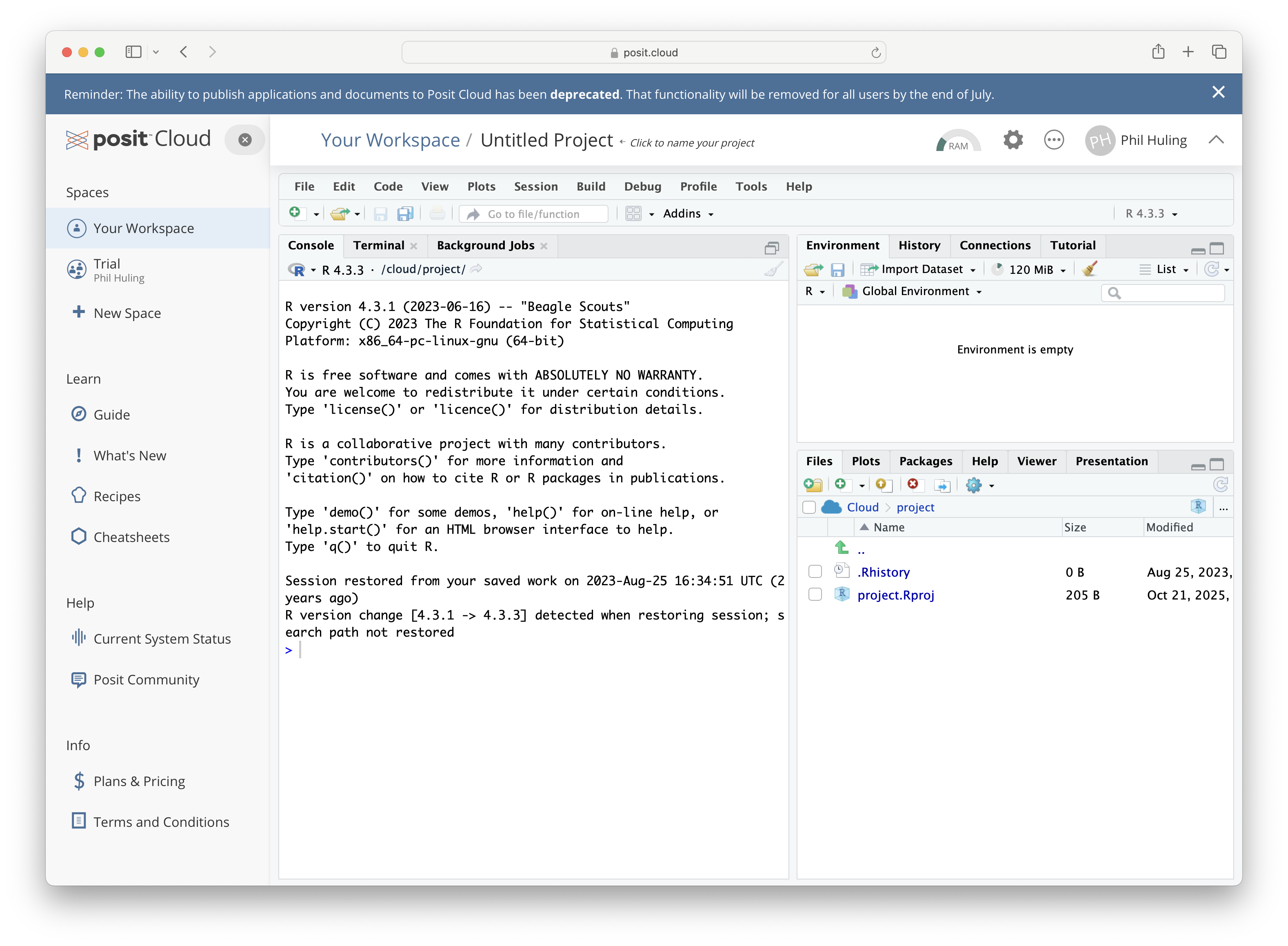
Figure 1.2: posit.cloud
While there are many good reasons to utilize the online posit.cloud option of RStudio, we will default to discussions on Statypus where we assume that the user is working with a downloaded copy. If you are struggling to utilize something on Statypus due to this issue, please check the help files at posit.cloud or email the author at phil.huling@slu.edu.
1.2 Using RStudio
RStudio is an improvement over the base R interface as it allows the user to view four different panes at one time. Users will primarily interact with RStudio in R “scripts” which appear in the upper left pane of the screen. Code the user wishes to run is then sent to the console which appears in the lower left pane of the screen. The upper right pane is typically used to view data and functions that the user has in their own personal environment at the moment, but can also be used to view a history of all lines of code that the software has run. The lower right pane is used for viewing plots, viewing and installing packages, as well as reading help files.
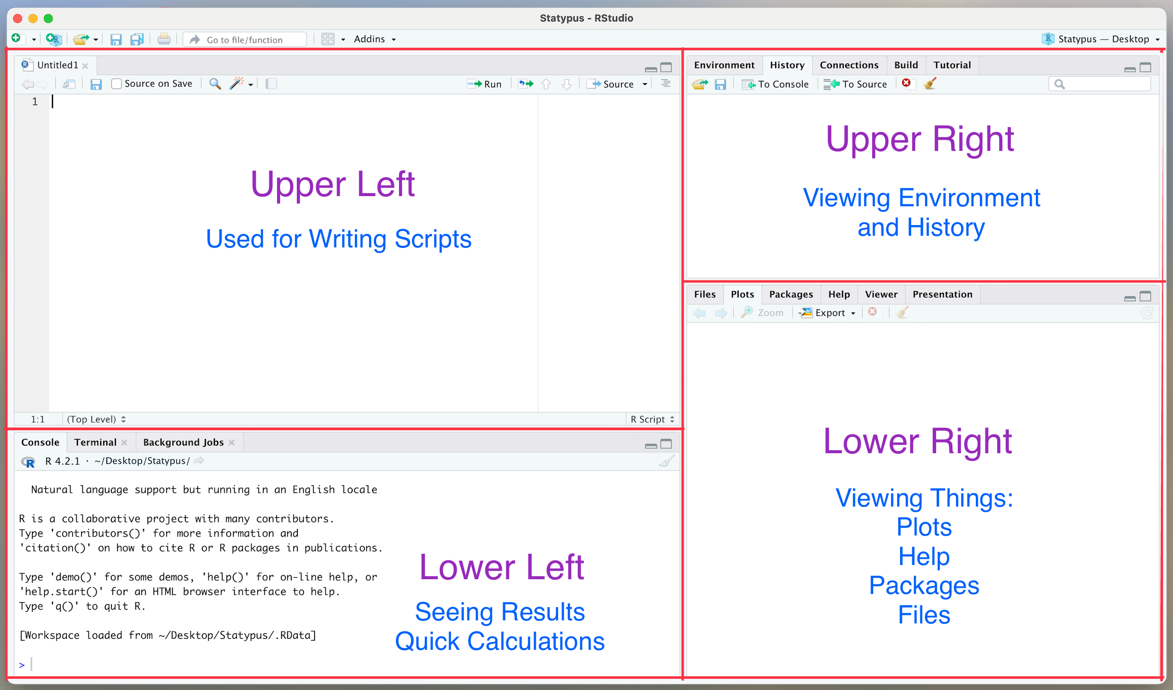
Figure 1.3: The 4 Panes of RStudio
The RStudio environment can be customized and manipulated. The above discussion is based on the default position and uses of the four panes present in the program.
New users may mistakenly try to use R through the R software directly. Doing so is definitely possible, but the use of RStudio is highly recommended. If you see a window like the one below, close that application and make sure you search your computer for “RStudio” and try again.
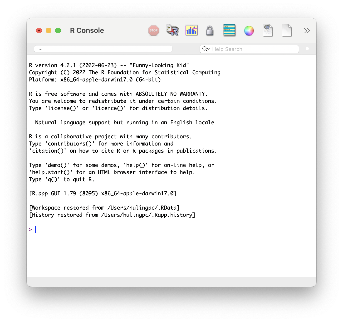
Figure 1.4: R GUI
The following video is a quick visual introduction to working within RStudio made by someone not affiliated with Statypus. It goes into more detail than is likely necessary, but is a very solid RStudio introduction video.
1.2.1 Left Panes
When we first launch RStudio, we may only see 3 panes. We will discuss how to get all four panes in Example 1.2 below. However, we can use the lower left pane to make quick calculations such as the one shown in the following example.
Example 1.1 (Our First Calculation) RStudio is a very robust program, so it is definitely capable of finding something as the square root of 4. To do this, we can invoke the sqrt() function. We will explain the use of functions more fully in Section 1.4. We will use a “New Function” box like the one below each time we introduce a new function.
The syntax of sqrt() is
where the argument is:
x: A numeric vector or array.
You can try this out by typing sqrt(4) into the Console or lower left pane of RStudio and then hit enter or return. The result of this is shown below.
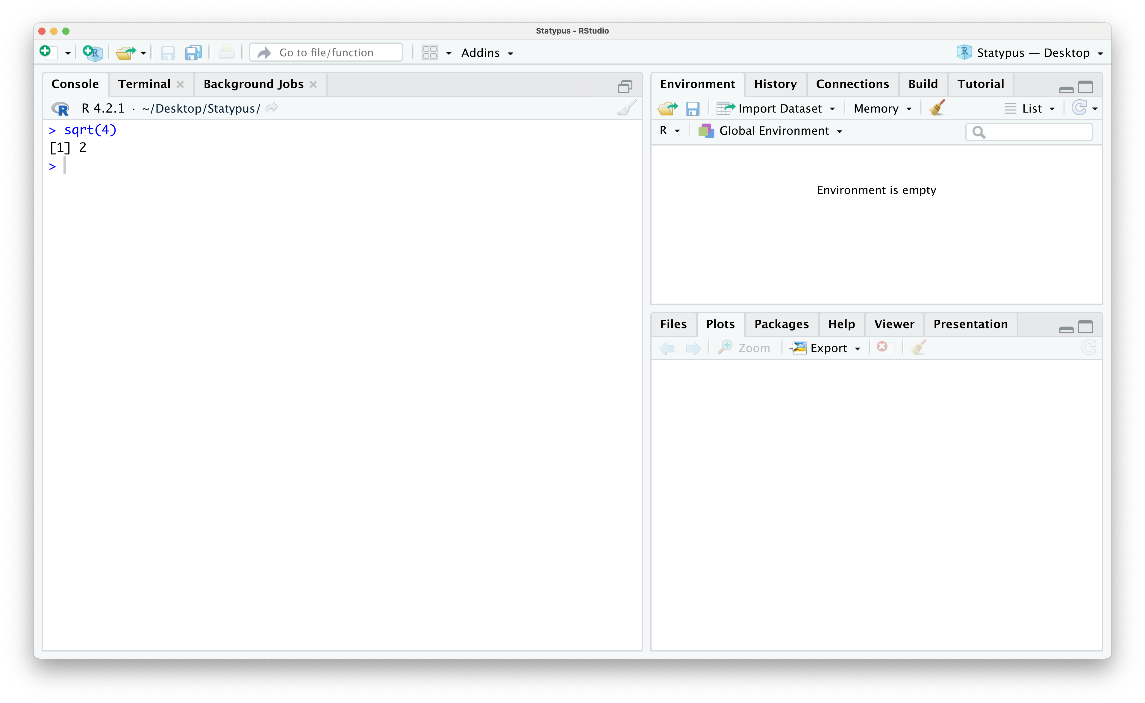
Figure 1.5: Our First Calculation
This tells us the result we expected, the (principal)10 square root of 4 which is 2.
The most common place you will interact with RStudio is in the upper left or source pane. We will primarily interact with files here called Scripts or R Scripts.
Definition 1.1 According to CRAN, a Script or “an R script is simply a text file containing (almost) the same commands that you would enter on the command line of R.” They will have a .R extension such as the file GoldenRatio.R we create in Example 1.3.
The “(almost)” in Definition 1.1 is a technical mention and not of concern to anything that will be done at Statypus. Unless you are planning on diving extensively into R, you can simply overlook that word and assume that an R script contains exactly the same commands you want to run.
Example 1.2 (Restoring the Fourth Pane)
In Figure 1.3 we showed that RStudio has 4 panes. However, launching RStudio will typically result in a screen like the one below for most people.
Figure 1.6: Missing the Fourth Pane
That isn’t four panes… there are only three panes. Where did the upper left pane go? RStudio does not always display the upper left pane upon startup. We can restore it in one of (at least) two ways. The simplest method that should work is to click on the “Pane Restore” icon. To find this icon, first locate the (likely grayed out) broom icon in the upper left hand corner of the Console pane which takes up the entire left side of RStudio currently. Directly above the broom you should see an icon that is two stacked windows which look like rectangles. This is shown below.
Figure 1.7: Restoring The Fourth Pane
An alternative method is a bit more manual, but more robust for the more advanced user as it allows you to choose what to populate the upper left pane with. If you click on the white rectangle covered by a white plus on a green circle icon in the upper left corner of the RStudio window, you should see the drop down menu shown below.
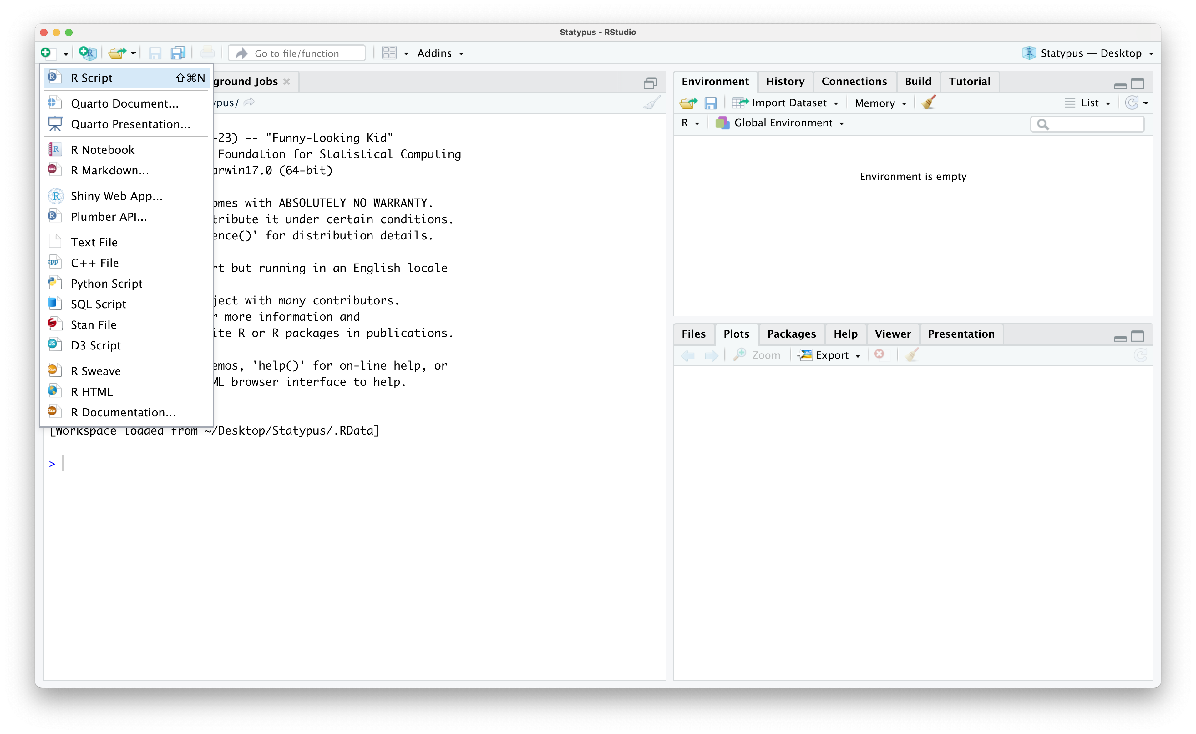
Figure 1.8: Restoring The Fourth Pane
Selecting “R Script” from this menu or using the “Pane Restore” icon should populate an R Script into the upper left pane and look like the screenshot below.
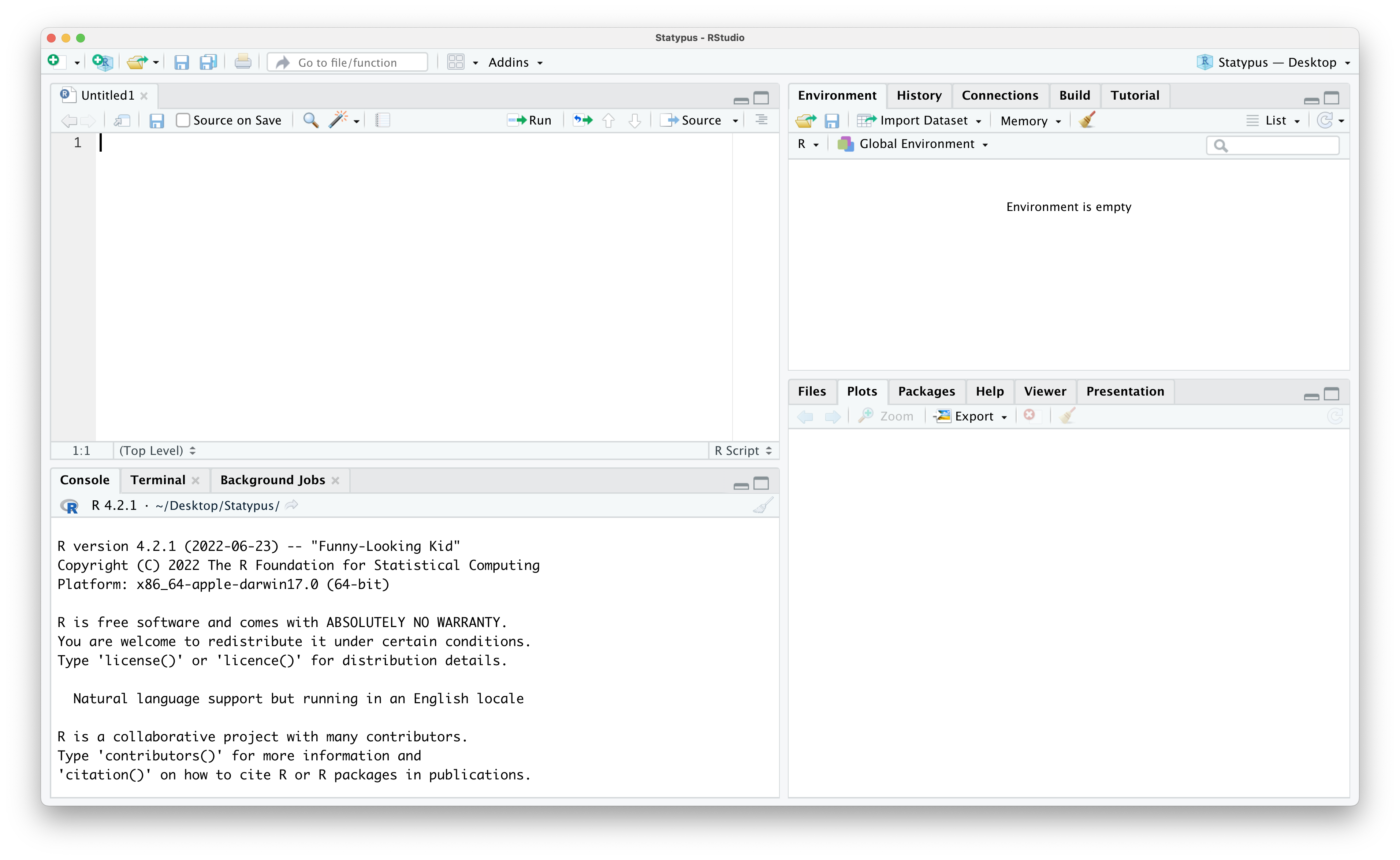
Figure 1.9: The Fourth Pane Restored
Example 1.3 (Creating Our First Script) In this example, we will create (and save) a script to calculate the famous mathematical constant known as the Golden Ratio11. The Golden Ratio is often denoted with the Greek letter \(\varphi\) (pronounced “fee” in most mathematical settings and like the “FI”12 in WI-FI at other times) and is given by the formula below.
\[ \varphi = \frac{1 + \sqrt{5}}{2}\]
The syntax needed to find an approximation of this value in R is given below.
If you hover your mouse over the upper right corner of the gray box above, a little “Copy to Clipboard” icon appear as shown below13:
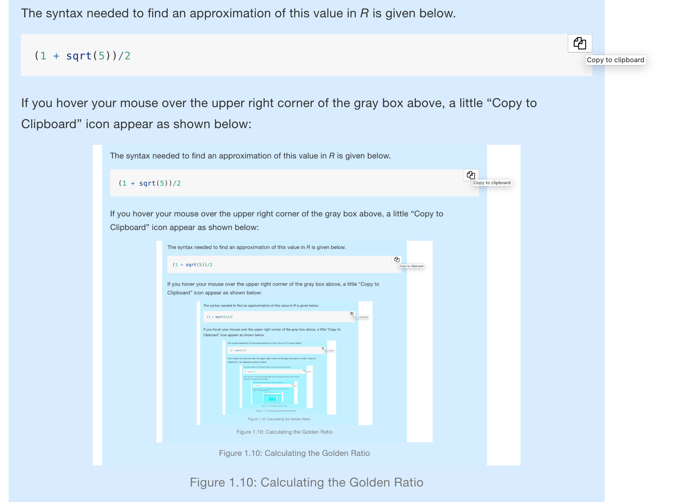
Figure 1.10: Calculating the Golden Ratio
Click on this and you now have the line of code above copied and ready to be pasted. If need be, open an R Script using the techniques shown in Example 1.2. If need be, put your cursor in the script by clicking on it and then paste the contents of the clipboard into your script with either Ctrl + V on a Windows machine or Command + V on an Apple machine (or numerous other options not covered here). You should now have something like the screen below.
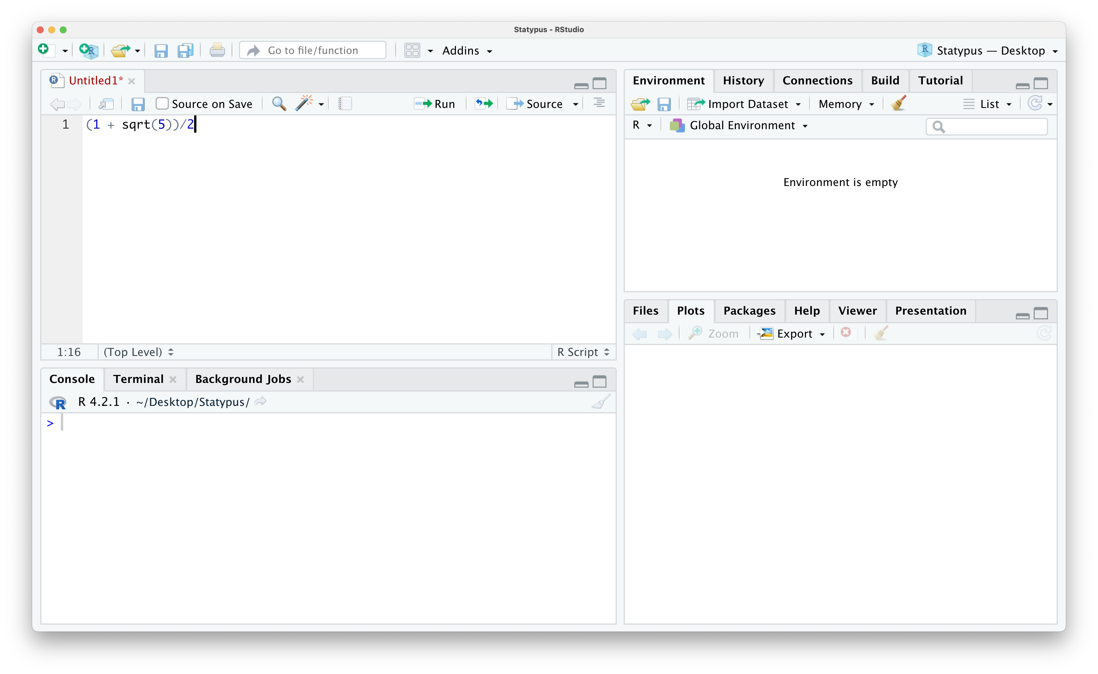
Figure 1.11: Calculating the Golden Ratio
If you simply hit enter or return you will get the following result.
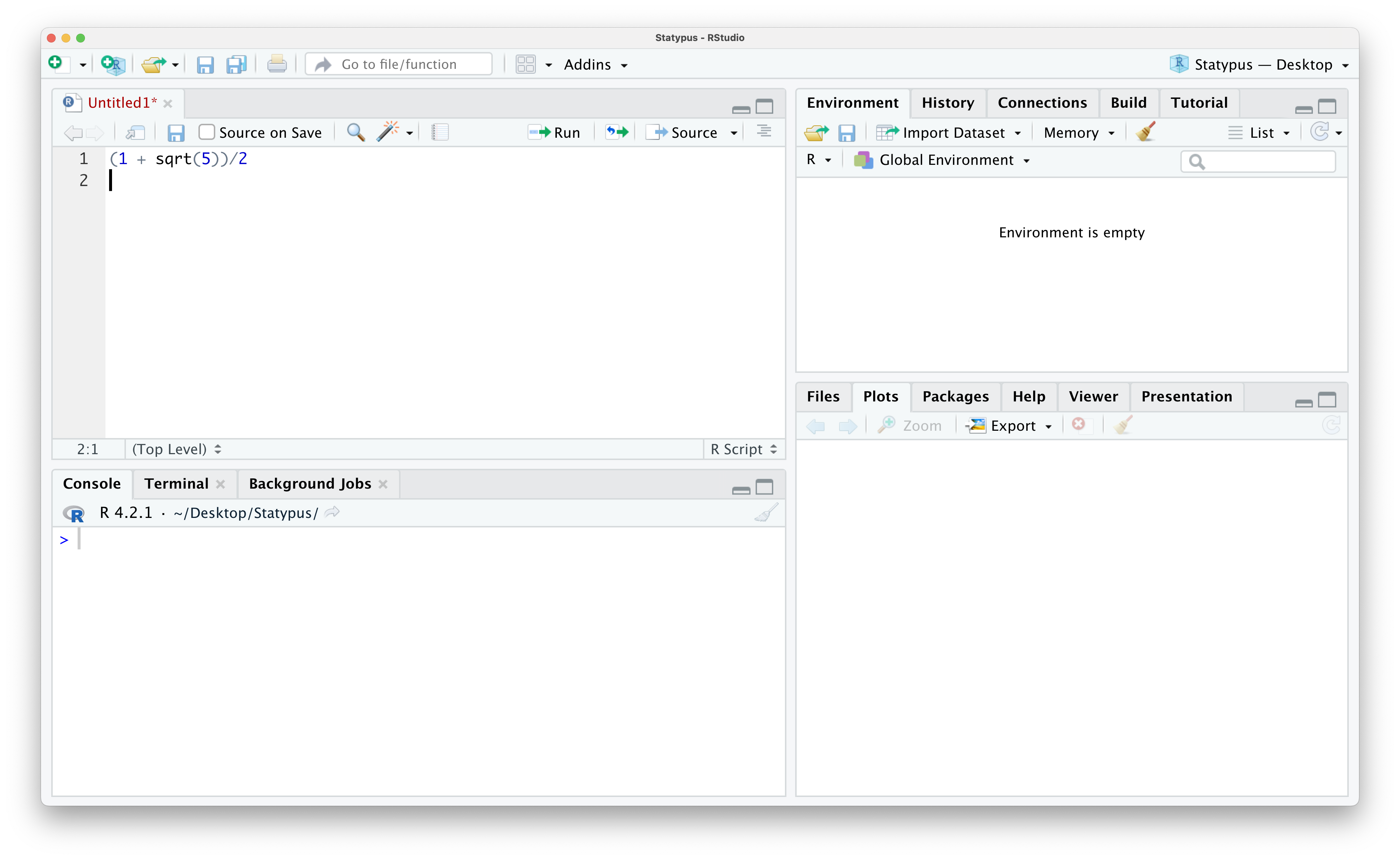
Figure 1.12: Calculating the Golden Ratio
Nothing happened other than the cursor moving down to the next line in our R Script. This is precisely what the enter/return key is designed to do! Note that R created a new line and labeled it with a 2 to the left noting that it is a new line. This is often helpful when working with others as you can say “Run Line 1” as compared to trying to point at their computer screen.
If we want to actually run this code, we have a couple of options. First make sure your cursor is on the line with the code you want to run, line 1 in this case. Then we can either hit Ctrl + enter/return on our keyboard or click on the “Run” icon in the bar directly above (and slightly to the right of) the code we just pasted in. Doing one of these should give you the result shown below.
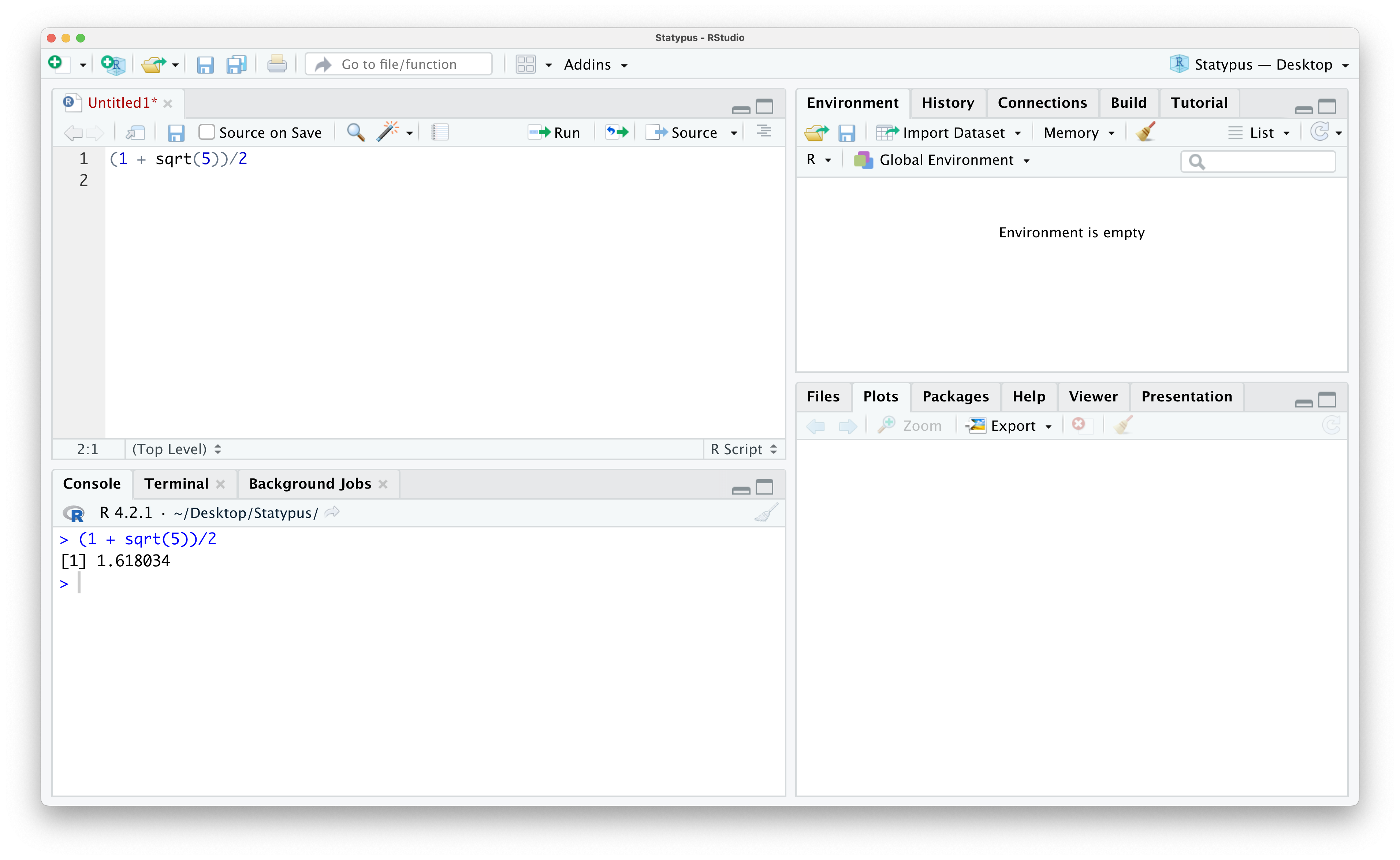
Figure 1.13: Calculating the Golden Ratio
One of the nicest features of scripts is our ability to save our work and make annotations. For example, if we wanted to leave a reminder of what this calculation was, we can put our cursor on line 2 and start by typing the character #14. Anything typed after this character on a line in an R script is a “comment” or “annotation” and will not affect the operation of code whatsoever. It can be used to remind yourself of what certain lines of code did or share information with others if you were to share your script with a classmate or colleague. Below we add a simple comment that we have found the Golden Ratio.
Figure 1.14: Annotating Our First Script
If you note in the image above, the name of the script is Untitled1 and it is currently displaying as red text. This indicates to the user that this script is currently not saved. To save the script, click on the “Save current document” icon which resembles a 3.5 inch diskette. If this is the first time you are saving a file, this brings up a dialog box where you can select the name you want to save the file as and also allow you to choose where to save it. Subsequent times clicking this icon will simply save the file with the current name in its current location.

Figure 1.15: Saving Our First Script
We now have a saved R script we could share with others showing how to calculate the Golden Ratio. While this example is not very exciting (especially statistically), it does show us the process for starting from a “fresh” opening of RStudio and ending with a shareable document.
The output we saw for the calculation given by (1 + sqrt(5))/2 in Example 1.3 above produced the output of [1] 1.618034 in the Console.
However, if we were to display that in this book without the use of screen shots, it would look something like this:
## [1] 1.618034The characters ## indicate that what follows is the output of R code. These characters are not part of the output, but simply a way that R communicates what is output when producing a document like this. You will see the ## characters preceding nearly every output in Statypus.
We glossed over where to save scripts in Example 1.3. RStudio has what is called a “Working Directory” where it will save files by default, but the user is free to choose where to save individual files anywhere they wish. We would recommend that you setup a folder somewhere convenient for you and save all of your R files there.
Example 1.4 When you are working in an R script, you should see a > prompt in the console as shown below.
Figure 1.16: The Annoying + Prompt
However, if you wanted to find the length of the longest river in the United States, you may try to run the following line of code.
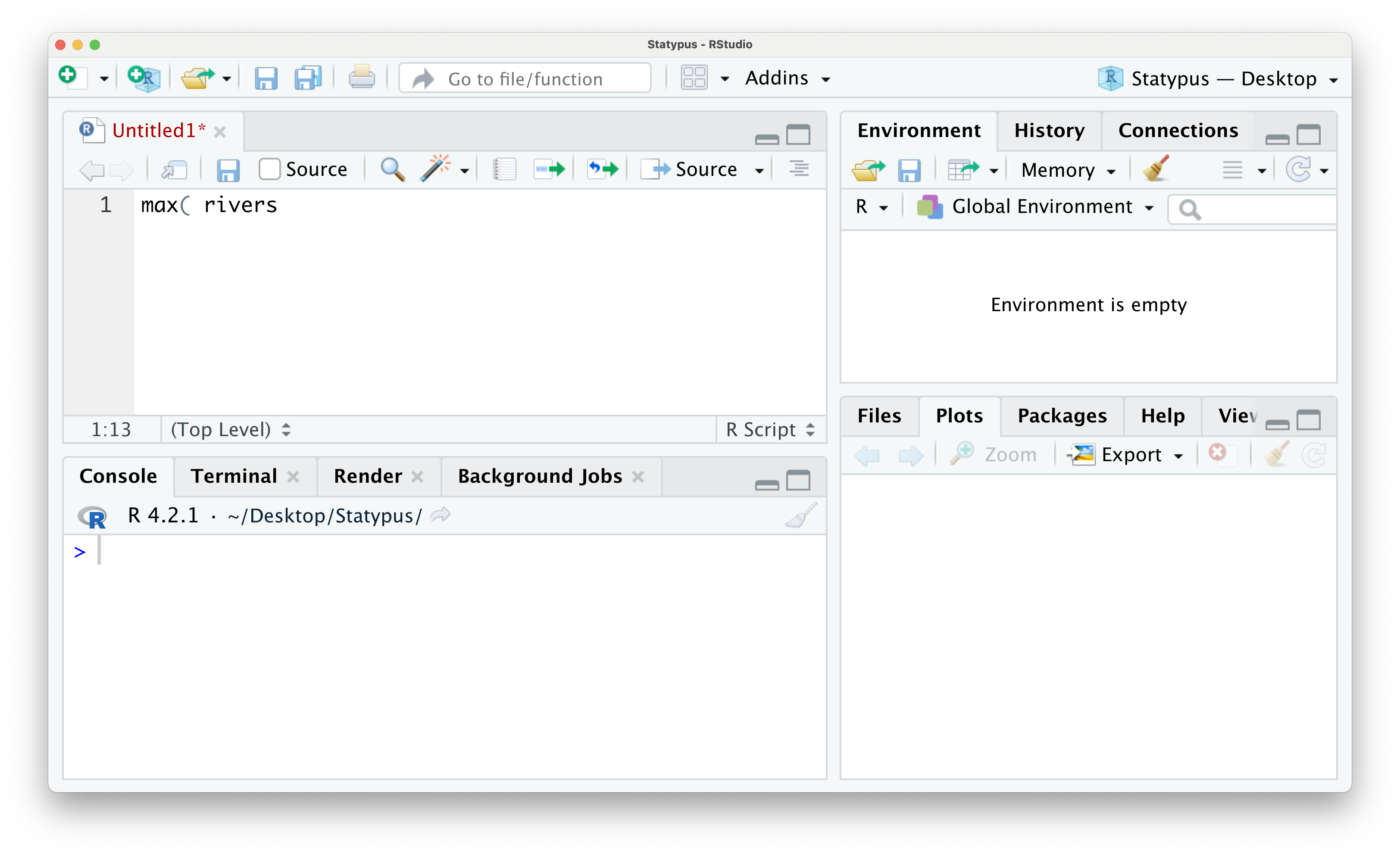
Figure 1.17: The Annoying + Prompt
If we run this line of code by either using the “Run” button or hitting CTRL + return, you will get the following outcome.
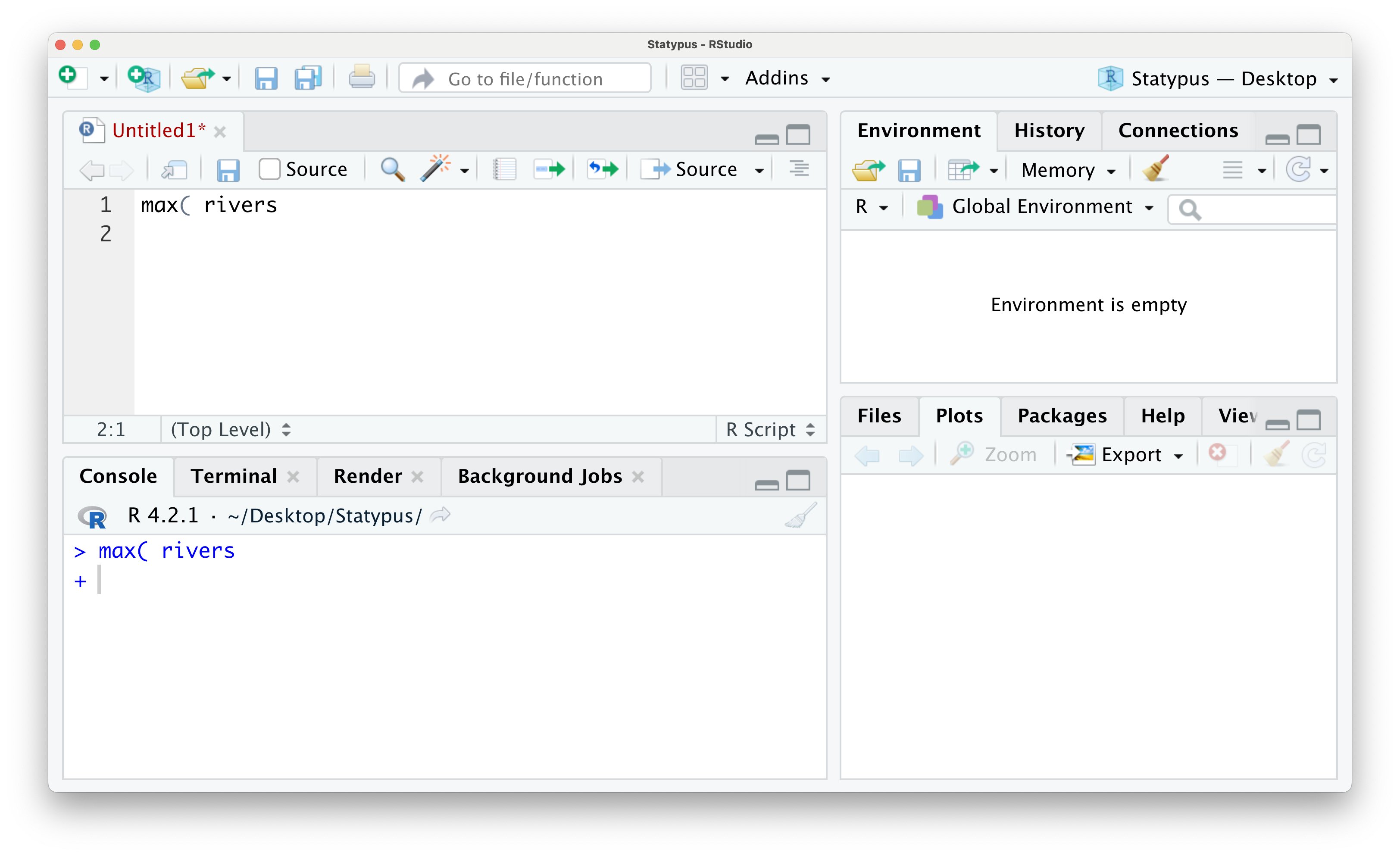
Figure 1.18: The Annoying + Prompt
We now have an unfamiliar + greeting us on the lowest line in the Console. This is RStudio’s way of telling you that it is awaiting more information. This is not an error and can actually be a tool for the advanced user, but it can frustrate beginning R students very easily. While you see the + prompt, you will be unable to run code normally from either the script or in the console. To escape this trap, the user need only put their cursor to the right of the + prompt and hit the esc key. The result of this is shown below.

Figure 1.19: The Annoying + Prompt
Once you have gotten the familiar > prompt back in the Console, you can place your cursor back into the script, fix or finish the code that caused the + prompt and then run the code. We show this below where all we fixed was closing the parentheses for the max function.
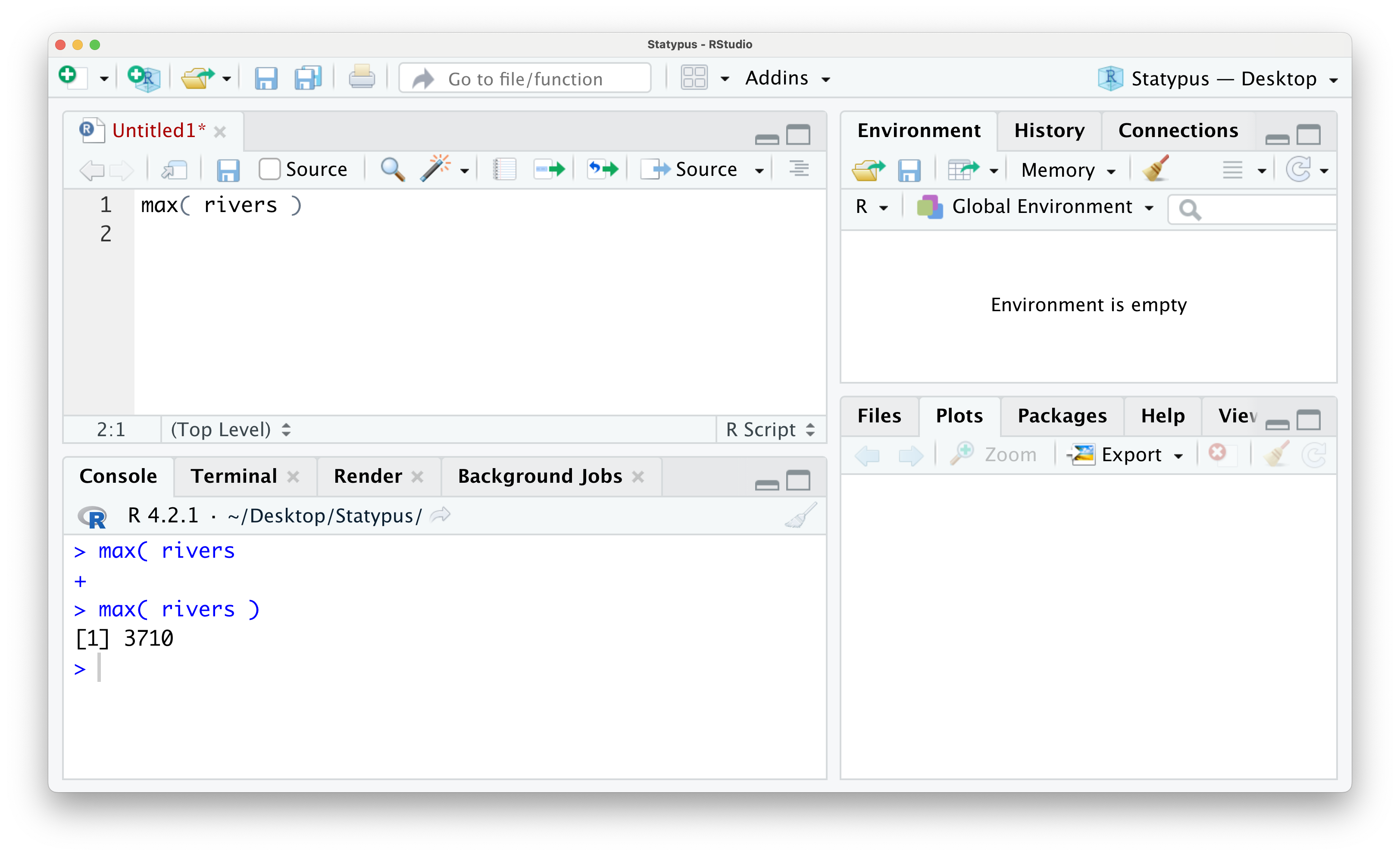
Figure 1.20: The Annoying + Prompt
We did not go into much detail about the rivers dataset which is built into R. You can run ?rivers in either a script of the Console if you want more information about this dataset. We will discuss the use of the ? more in Section 1.5.1.
1.2.2 Right Panes
Thus far, our entire interaction with RStudio has been via the left panes. The right panes will be used for a variety of reasons. Both the upper right and lower right pane have multiple uses which can be changed via the tabs at the tops of the panes. We will begin by examining the major uses of the upper right pane first
Example 1.5 The most prevalent use of the upper right pane of RStudio is the Environment. The Environment shows any data or user defined functions which have been loaded or created. For example, if we continue the work done in Example 1.3, we could save the value of \(\varphi\) we calculated so that it could be used in future calculations without needing to type out the full formula again. We will save it with the spelling of the Greek letter \(\varphi\), phi. We will go deeper into the use of the “back arrow” in Section 1.3.2, but for now, the following line of code will store the value we calculated earlier into a variable named phi.
Below we show the result of adding this line of code to the R script we created in Example 1.3.
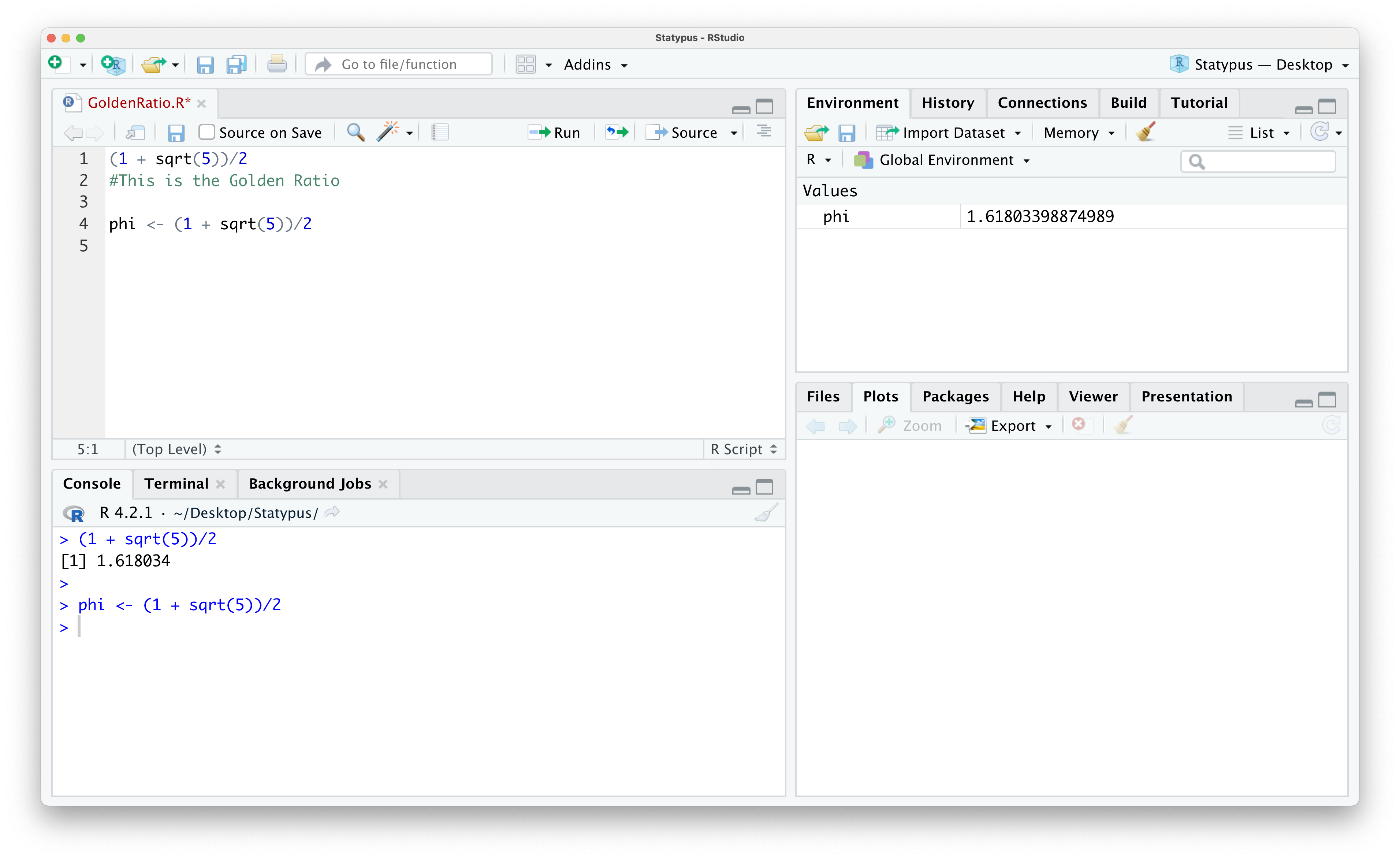
Figure 1.21: Looking at Data in the Environment
Note that R did not show the value of phi in the console, but it now does show that we have phi in the Environment and it shows the value of it there as well. Once we have a value saved in our Environment, we can then do arithmetic with it just like we would with a number like 7. For example, we could run the following block of code to find the sum of \(\varphi\) and 2.
## [1] 3.618034The second most common use of the upper right pane is the History tab. If you click on that, you see a list of all the commands you have run on RStudio. Here you can search for different commands you have run. If you looked at the environment used to create the GoldenRatio script, you would see the following.
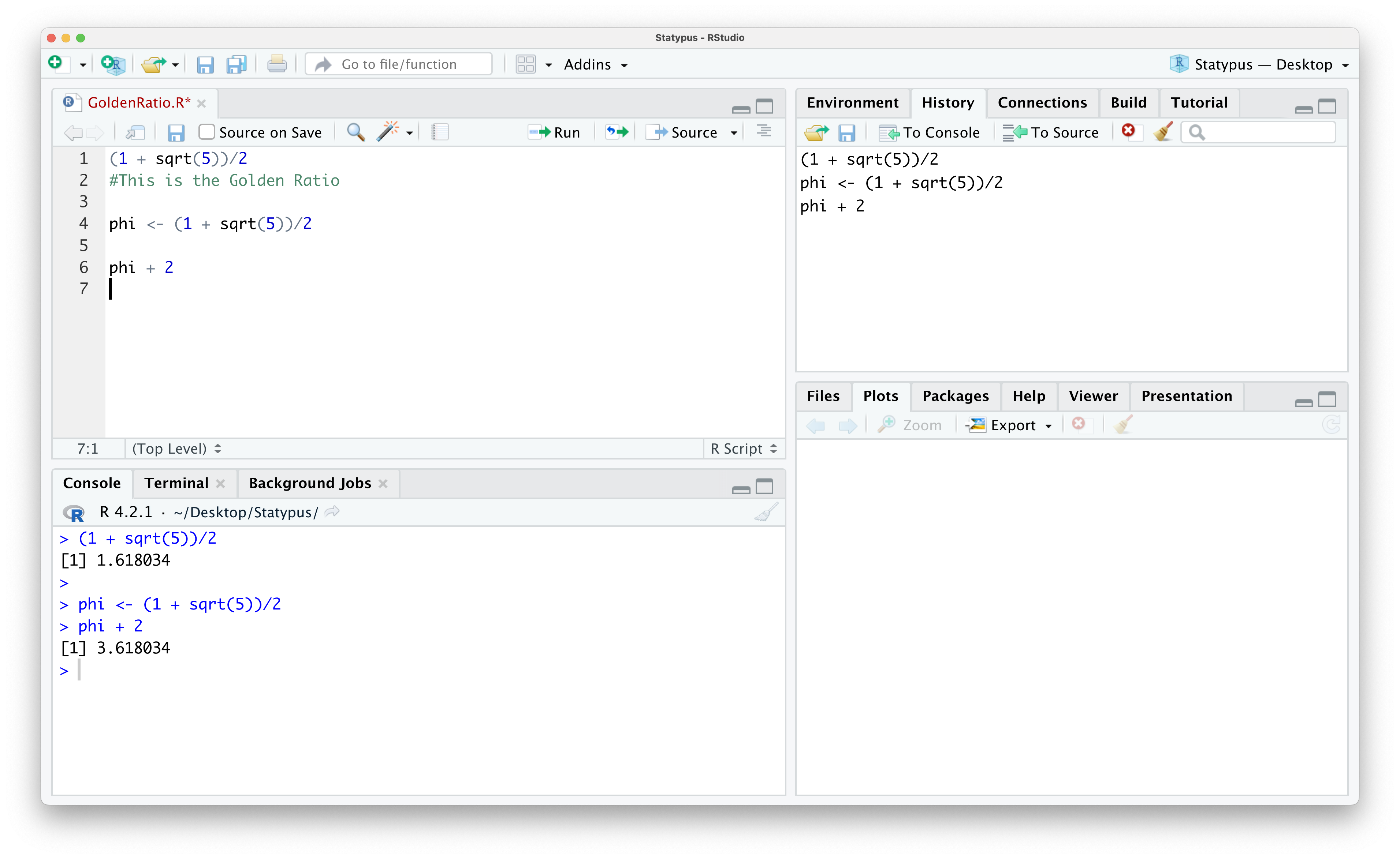
Figure 1.22: Looking at the History Tab
The most common way we will use the lower right pane is for plots. We look at a simple example below.
Example 1.6 We first saw the built-in dataset rivers in Example 1.4. According to RStudio:
| “This data set gives the lengths (in miles) of 141 “major” rivers in North America, as compiled by the US Geological Survey.”
We won’t get into a detailed analysis of it here, but we will look at a histogram of the dataset. We will not introduce this function until Chapter 3, but we use it now to simply produce a plot we can view. If you copy and paste the following line of code into the Console, you should get a result like the following.
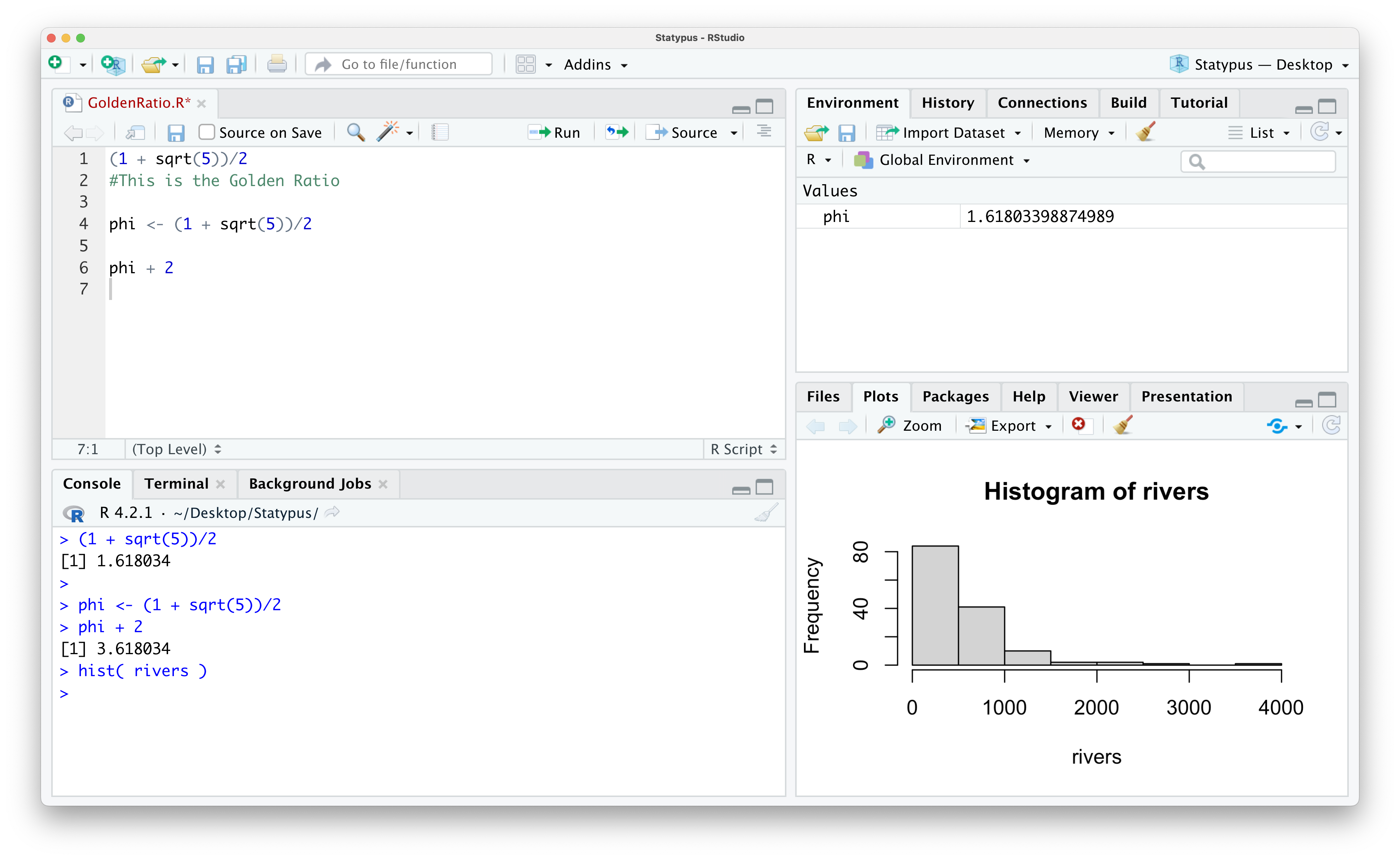
Figure 1.23: Our First Plot
This shows that most rivers have a length of no more than 500 miles and only a few have a length of over 2000 miles. As mentioned already, we will further investigate histograms and the hist() function in Chapter 3.
1.3 Data
In Example 1.5, we saved the value of the Golden Ratio to our Environment with the following line of code.
This was our first time saving data to our device using R. We used the left arrow operator <- to save the value of (1 + sqrt(5))/2 into a value which we called phi. The left arrow operator will be our primary way of storing or saving data to our device.
Example 1.7 We can save the value of 2 to have the name two with the following line of code:
There is absolutely no reason someone would want to do this, but it does show how one can store a numeric value to a chosen name in a way that is hopefully so simple that it isn’t forgotten.
In Example 1.7, we saved the value of 2 to a value called two. Built into R is an approximation of the mathematical constant \(\pi\). We can find this by typing pi into RStudio and running that line.
## [1] 3.141593If someone15 wanted to change the value of pi to be 3.2 what line of code would you need to run in R?
If you successfully changed the value of \(\pi\) in the above “Now it’s your turn!,” you should really “undo” that with the remove function, rm(). To do this, simply run the following line of code.
We note that this will not actually remove the constant from your machine, but it will only remove the “new” copy of pi that we created.
We will revisit the remove function later in Example 1.30 in Section 1.5.6.
1.3.1 Basic Data Types
When R stores data, it puts it into certain types. The types we will study here on Statypus are
- Numerical
- Character
- Logical
We will look at these types in the following example.
Example 1.8 The following code block shows the storage of three different types of values called googol, bloodType, and maybe.
Below shows the way these values would display in your Environment.
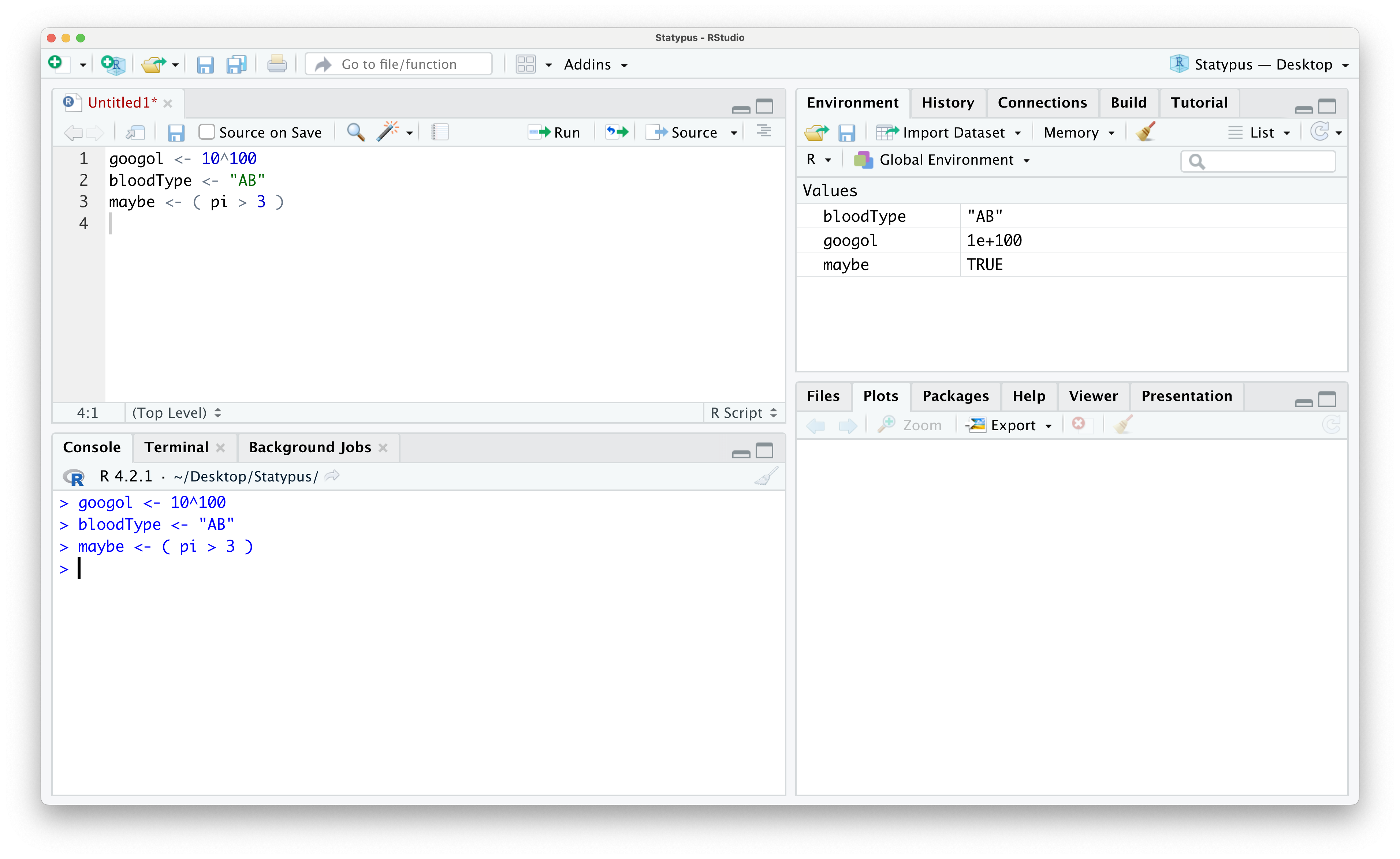
Figure 1.24: Looking at Data in the Environment
The value googol represents the actual number named googol16 and it is stored in scientific notation. The notation 1e+100 represents the number \(1 \cdot 10^{100}\). This is numeric data.
The value bloodType represents a patient’s blood type being "AB" and is saved as the character type is often called a character string. Please note the quotation marks around the string and see the remark below.
The final value is called maybe and the value shown in the Environment is TRUE. This is because it is the result of the statement ( pi > 3) which is a true statement. This is an example of the logical data type. Logical data can take on one of two values, True or False, but in R they must be written as TRUE or FALSE.
It is very important to note that when we saved the blood type in Example 1.8 that we contained the character string in quotation marks. Failure to do so will cause an error and we will see the result of this in Example 1.21 in Section 1.5.3.
Unless you have redefined the values of T or F, these values are shortcuts to the values of TRUE and FALSE respectively.
Most people begin their interaction with variables using the letter \(x\) for everything. The phrase “Solve for \(x\)” can even cause trepidation in some hearts. We are certainly able to use \(x\) here, but we note that it will appear as x in R.
However, R allows us the flexibility to name variables nearly anything we want. For example, in Example 1.3 we used the variable name phi for the Greek letter \(\varphi\). In Chapter 4 we will introduce the sample mean which we will denote \(\bar{x}\) which is read as “\(x\)-bar” and we will store values in RStudio as xbar.
In general, you should use variable names that are descriptive and representative of what they are labeling. There are a few rules, however. Variable names cannot begin with a number or a “dot”17, .. You can combine words with juxtaposition such as MeanOfSample or MassOfSpring or with the underscore character, _, such as Mean_Of_Sample or Mass_Of_Spring.
We will introduce Data Frames in Section 1.3.4 and at times will save a copy of a data frame we are working with as df or dd to simplify or shorten some code. We call this a Working Copy of a data frame and discuss it in Section 1.5.6
Choose your variable names with care, however, as variable names are case sensitive. We discuss this in a Big Idea at the beginning of Section 1.5.2.
You should not use variable names that could conflict with existing R objects. These can be single letters as below.
Do not use: c, q, t, C, D, I, T, F
These letters have built in uses within R and assigning variables to them can cause issues. Further, certain names should be avoided as they may align with functions such as the ones below.
Do not use: sample, sum, mean
1.3.2 Vectors
It seems obvious that we won’t get very far having to give a unique name to each piece of data we have and that it would make more sense to give a name to a collection of data values. If those pieces of data are of the same type as discussed in Section 1.3.1, then the result is what is called a vector.
Definition 1.2 A Vector is an ordered collection of values of a similar type of data. Each value in a vector is known as an Entry and the position of each entry is known as the entry’s Index or Indices if dealing with more than one index. The total number of entries is known as the Length of the vector. The first entry has an index of 1, the second entry has an index of 2, and finishes with the last entry having an index matching the length of the vector.
Vectors are most easily created by using the function c() which combines or concatenates the objects passed to it.
The syntax of c() is
where the arguments are objects to be concatenated. All NULL entries are dropped unless at the very beginning of the argument list.
We will illustrate this via Example 1.9 where we will setup our first real dataset. However, we will first introduce the Left Arrow Operator.
Definition 1.3 The Left Arrow Assignment Operator or simply the Left Arrow Operator, <-, is used to assign a value to a name. It can be created by combining the less than character < with a dash -. We recommend that you place a space before and after the left arrow operator.
There is a bit of a debate about whether to use the left arrow operator, <-, or a single equal sign, =. While the two are nearly interchangeable, there are places where = cannot be used and on Statypus we will only use = for defining arguments within functions or when we define variables before a block of code where we want to mirror the idea of a function.
In addition, using the left arrow operator makes a clear distinction on where the value and name should be in relation to the operator. While x = 2 is equivalent to x <- 2, look what happens if we reverse the order.
## Error in `2 = x`:
## ! invalid (do_set) left-hand side to assignment
R was unable to complete our request and gave us an Error, a topic we will more fully investigate in Section 1.5.3.
The advanced reader may wonder about a potential Right Arrow Assignment Operator and such an operator does indeed exist. While 2 <- x will cause an error, we could use the code 2 -> x successfully. While there is nothing wrong with using this operator, we have made a choice to not use it within the pages of Statypus. This will require the code to be consistent where the name appears on the left hand side of the assignment operator and the value appears on the right hand side. Consistency is required to gain familiarity.
Example 1.9 (Snickers: Part 1) This example is the first of a few examples where we will play with a vector of numeric values called snickers. The reader can see Section 6.7.2 to get more information about this dataset. Copy and paste the code from the following “Data Download” box into an R script or the R Console and run it to load snickers into your Environment.
Use the following code to store the variable snickers.
snickers <- c(
51.1, 53.8, 51.1, 53.8, 51.9, 52.5, 53.2, 53.8, 52.4, 54.0,
53.5, 54.4, 51.1, 52.4, 50.8, 52.1, 51.9, 51.2, 52.7, 53.3,
52.1, 54.1, 52.7, 54.1, 51.9, 53.7, 52.2, 53.7, 54.2, 52.2,
52.5, 54.5, 53.0, 51.9, 54.4, 54.7, 53.0, 53.8, 54.3, 53.3,
52.4, 51.2, 53.5, 52.4, 52.3, 55.2, 51.2, 54.3, 53.3, 51.9,
51.3, 53.8, 53.3, 52.0, 50.3, 51.8, 51.1, 52.6, 52.5, 53.9,
53.1, 53.9, 52.9, 52.2, 50.5, 52.5, 50.3, 52.2, 52.2, 51.7,
52.0, 52.5, 53.1, 53.8, 54.0, 53.4, 52.3, 50.9, 53.9, 53.4,
53.4, 52.5, 53.6, 53.0, 56.2, 54.2, 52.5, 52.4, 53.3, 52.9,
51.8, 50.9, 52.3, 54.0, 51.2, 53.6, 51.1, 50.3, 53.2, 52.6
)
The result of loading snickers should result in a screen like the one below. Note that we now see snickers listed in the Environment where we saw things like phi or googol earlier.
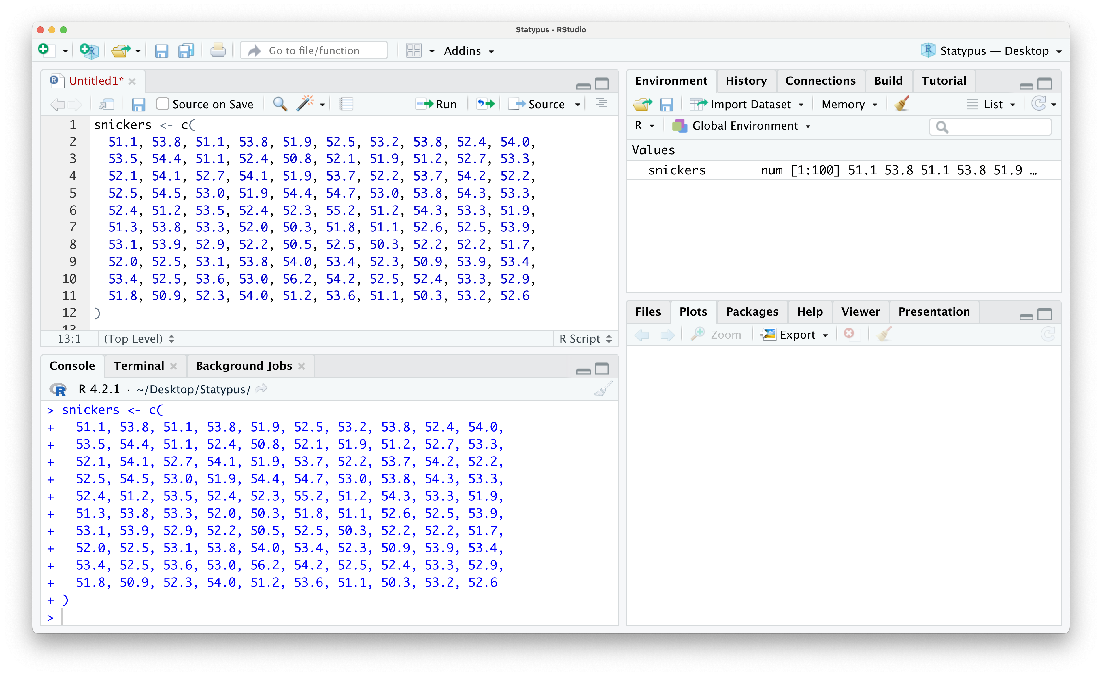
Figure 1.25: Looking at Data in the Environment
The simplest thing we can do with a vector is to have R display it for us by simply typing out the variable’s name and running that line of code. If you do this, you will get the following output.
##   [1] 51.1 53.8 51.1 53.8 51.9 52.5 53.2 53.8 52.4 54.0 53.5 54.4 51.1 52.4 50.8
##  [16] 52.1 51.9 51.2 52.7 53.3 52.1 54.1 52.7 54.1 51.9 53.7 52.2 53.7 54.2 52.2
##  [31] 52.5 54.5 53.0 51.9 54.4 54.7 53.0 53.8 54.3 53.3 52.4 51.2 53.5 52.4 52.3
##  [46] 55.2 51.2 54.3 53.3 51.9 51.3 53.8 53.3 52.0 50.3 51.8 51.1 52.6 52.5 53.9
##  [61] 53.1 53.9 52.9 52.2 50.5 52.5 50.3 52.2 52.2 51.7 52.0 52.5 53.1 53.8 54.0
##  [76] 53.4 52.3 50.9 53.9 53.4 53.4 52.5 53.6 53.0 56.2 54.2 52.5 52.4 53.3 52.9
##  [91] 51.8 50.9 52.3 54.0 51.2 53.6 51.1 50.3 53.2 52.6
The expression [16] on the second line of the output above tells us that 52.1 is the 16th value (of the 100 chocolate bars) of the snickers vector.
We also show a screenshot of what this looks like below.
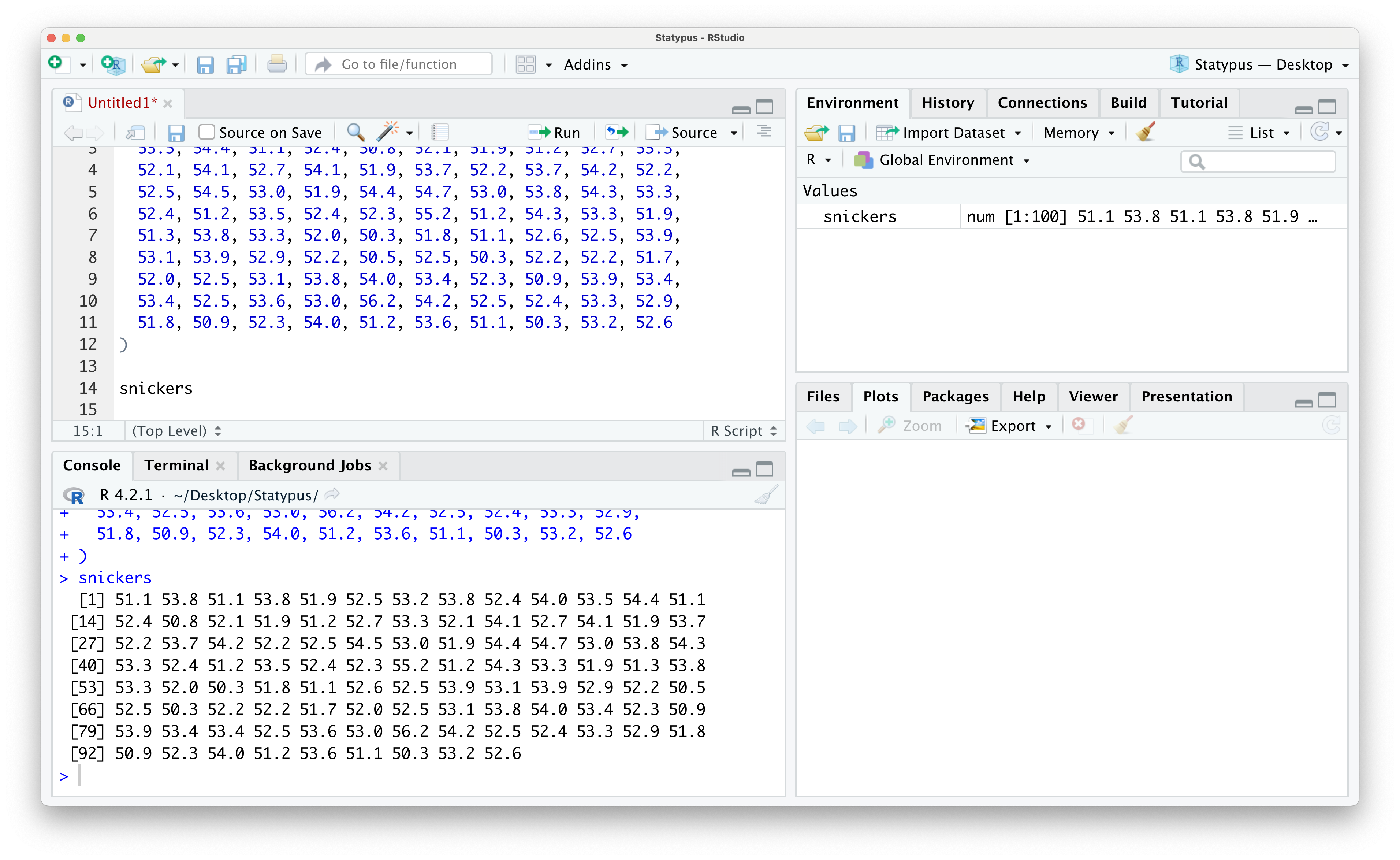
Figure 1.26: Looking at Data in the Environment
This is an example of Raw Data and it is not even ordered in anyway that is useful for the user. We can use the sort() function (which we will explain in more detail in Chapters 3 and 4) to see the mass of the chocolate bars starting with the most massive.
##   [1] 56.2 55.2 54.7 54.5 54.4 54.4 54.3 54.3 54.2 54.2 54.1 54.1 54.0 54.0 54.0
##  [16] 53.9 53.9 53.9 53.8 53.8 53.8 53.8 53.8 53.8 53.7 53.7 53.6 53.6 53.5 53.5
##  [31] 53.4 53.4 53.4 53.3 53.3 53.3 53.3 53.3 53.2 53.2 53.1 53.1 53.0 53.0 53.0
##  [46] 52.9 52.9 52.7 52.7 52.6 52.6 52.5 52.5 52.5 52.5 52.5 52.5 52.5 52.4 52.4
##  [61] 52.4 52.4 52.4 52.3 52.3 52.3 52.2 52.2 52.2 52.2 52.2 52.1 52.1 52.0 52.0
##  [76] 51.9 51.9 51.9 51.9 51.9 51.8 51.8 51.7 51.3 51.2 51.2 51.2 51.2 51.1 51.1
##  [91] 51.1 51.1 51.1 50.9 50.9 50.8 50.5 50.3 50.3 50.3
While this is still a lot of information to try and digest, at least we can easily tell that the most massive chocolate bar had a mass of 56.2 grams and the least massive came in at 50.3 grams.
Since many datasets can have enough entries that it becomes impossible to display them on the user’s computer screen, it would be helpful if we could easily request R to just show us the first few values of a dataset. We can use the head() function to do just this.
The syntax of head() is
where the argument is:
x: An R object.
Example 1.10 (Snickers: Part 2) We can continue our investigation of the snickers dataset by seeing how head() works when applied to it.
## [1] 51.1 53.8 51.1 53.8 51.9 52.5As you can see, as compared to simply running snickers like we did in Example 1.9, the code head( snickers ) simply displays the first 6 entries of snickers allowing us to see a few prototypical values of the dataset without scrolling our screen.
Another helpful function for examining a dataset is the structure function, str().
The syntax of str() is
where the argument is:
object: Any R object about which you want to have some information.
To see what str() offers us, we will return to our snickers data.
Example 1.11 (Snickers: Part 3) Let’s just see what happens when we run str() on snickers.
## num [1:100] 51.1 53.8 51.1 53.8 51.9 52.5 53.2 53.8 52.4 54 ...What we see is that snickers contains data of the num or numeric type and it has indices from 1 to 100. This is similar to the information about the dataset contained in the Environment as shown below.
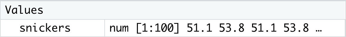
Figure 1.27: Looking at Data in the Environment
We will use str() for objects other than vectors and remind the reader that this is a great function to use if you happen to forget what a variable represents and it’s not easily found within your Environment.
We will actually deal with two types of numerical data. For example, in Example 1.11, we saw that the snickers dataset was a vector of length 100 containing numeric values as indicated by the num in either the output of str( snickers ) or as seen in the environment as shown in Figure 1.27. If the numeric data we are dealing with only contains integers, it may actually be of the int or integer type. Fortunately, the user does not need to worry about the distinction and R will do calculations with both types simultaneously without the user ever knowing.
Note that Definition 1.2 explicitly requires all entries have the same data type. If you attempt to combine mixed varieties of data with c(), R will do its best to create a vector of a single type. Turning numeric values into character strings is one of the most likely outcomes of trying to mix data types. For example, consider the code below trying to combine 1 and the letter "B".
## [1] "1" "B"To avoid the conflicting types of data, R automatically turned the numeric value of 1 into the character string "1" as we see in the output.
If we saved this vector as vec with the following code
would show the following in the environment making it clear that vec is a vector of character strings.
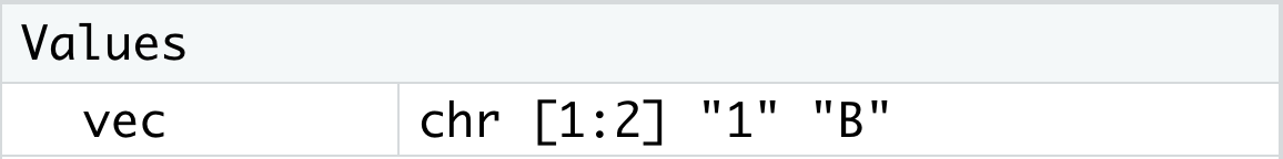
Figure 1.28: Looking at Data in the Environment
We loaded the snickers dataset in Example 1.9 and mentioned in subsequent examples that it is a vector of 100 numeric data values. As we mentioned in Definition 1.2, each entry of a vector has an index, and the indices of snickers are from 1 to 100. To extract a single entry or multiple entries, we will append a set of brackets [ ] after the vector name. This set of brackets is called the bracket operator.
Definition 1.4 The bracket operator can be applied to vectors and other data formats to extract or replace parts.
Example 1.12 To extract the first entry of snickers we use the bracket operator shown in the following line of code.
## [1] 51.1To extract the fifteenth entry of snickers we use the following line of code.
## [1] 50.8To extract the first 12 entries of snickers we would use the bracket operator as follows where mention that if a and b are integers, then a:b is a quick way to give the vector of all integers from a to b.
## [1] 51.1 53.8 51.1 53.8 51.9 52.5 53.2 53.8 52.4 54.0 53.5 54.4Using a “hidden” logical vector (which we will discuss in a “Big Idea” directly after this example), we can also extract only the values of snickers that are less than 51 by inserting an inequality within the bracket operator.
## [1] 50.8 50.3 50.5 50.3 50.9 50.9 50.3From this, we can see that there were only 7 snickers bars in the sample that had a mass of less than 51 grams.
In Example 1.12, use used the bracket operator with an enclosed inequality to extract just those entries that satisfied the inequality snickers < 50. To see how this works, we look at what happens if we just run the inequality in RStudio.
##   [1] FALSE FALSE FALSE FALSE FALSE FALSE FALSE FALSE FALSE FALSE FALSE FALSE
##  [13] FALSE FALSE  TRUE FALSE FALSE FALSE FALSE FALSE FALSE FALSE FALSE FALSE
##  [25] FALSE FALSE FALSE FALSE FALSE FALSE FALSE FALSE FALSE FALSE FALSE FALSE
##  [37] FALSE FALSE FALSE FALSE FALSE FALSE FALSE FALSE FALSE FALSE FALSE FALSE
##  [49] FALSE FALSE FALSE FALSE FALSE FALSE  TRUE FALSE FALSE FALSE FALSE FALSE
##  [61] FALSE FALSE FALSE FALSE  TRUE FALSE  TRUE FALSE FALSE FALSE FALSE FALSE
##  [73] FALSE FALSE FALSE FALSE FALSE  TRUE FALSE FALSE FALSE FALSE FALSE FALSE
##  [85] FALSE FALSE FALSE FALSE FALSE FALSE FALSE  TRUE FALSE FALSE FALSE FALSE
##  [97] FALSE  TRUE FALSE FALSE
We see that the result is a vector of logical values where the \(k^\text{th}\) entry is the logical result of testing if the \(k^\text{th}\) entry of snickers is strictly less than 51. For example, snickers[ 1 ] was 51.1 which is not less than 51 so the first entry of this new vector is FALSE. Moreover, snickers[ 15 ]was 50.8 which is less than 51 so the fifteenth entry of the above logical vector is TRUE. When we put this logical vector into the brackets after snickers, it will keep the entries with indices that are TRUE and omit the values that are FALSE.
You can use the following logical “test operators” to do similar tests:
>: Tests if the left hand side is strictly greater than the right hand side.<=: Tests if the left hand side is less than or equal to the right hand side.>=: Tests if the left hand side is greater than or equal to the right hand side.==: Tests if the left hand side is equal to the right hand side.!=: Tests if the left hand side is not equal to the right hand side.
Extract the list of the snickers bars that were exactly the labeled mass of 52.7 grams.
Extract the list of snickers that were at least 54 grams.
Extract the \(40^\text{th}\) to \(47^\text{th}\) entries of
snickers.
Insert solution video here
Example 1.13 We can actually perform arithmetic calculations with vectors. To begin the discussion, we will define two vectors, x and y.
We can begin by seeing what happens if we add 17 to x via the following line of code.
## [1] 18 19The result is the sensible result of adding 17 to each entry of x.
Another simple things we could do is to multiply y by 1318 using the star operator, *, via the following line of code.
## [1] 39 52 65The result is again the sensible result of 13 multiplied by each entry of y.
We could also combine the vectors with the c() function.
## [1] 1 2 3 4 5Here we see that c() created a new vector by combining or concatenating the elements of x with the elements of y. We could similarly combine them as follows.
## [1] 3 4 5 1 2This shows that c() maintains the order the user provides and combines them. We can also use c() to add a single entry to either vector. For example, we could add the entry 6 to y with the following line of code.
## [1] 3 4 5 6In addition, we can use the bracket operator along with the left arrow assignment operator to change values in a vector. For example, if we wanted the first entry of y to be 1818 for some reason, the following lines of code will accomplish that and print the result to confirm what we have done.
## [1] 1818 4 5Most arithmetic and algebra books allow juxtaposition to be used for a short hand for multiplication. For example, in most math classes we take the symbols \(13y\) to mean 13 times the variable \(y\). However, this does not work in R. Moreover, attempts to use a space between the values, 13 y, or to use parentheses, 13(y), will also fail to give the desired product.
You must use the star operator to multiply objects in R.
Note that none of the lines of code in Example 1.13 modified the value of x or y and none of the outputs were saved for future work. If we wanted to save the result of combining x and y, we could have used a line of code like the following
which creates a new vector called z. We can look in the Environment or run the single line of code below to confirm that z is the vector we expect.
## [1] 1 2 1818 4 51.3.3 Downloading Data
When we loaded snickers in Example 1.9, we had to contain all of the values in the vector in the line of code we ran. This is highly impractical as some datasets contain information about more than one type of data type and can contain hundreds if not hundreds of thousands (or more) of entries. We will typically work with data that is already saved in a way that R can easily use it. The primary file type we will use on Statypus is a CSV File.
Definition 1.5 A CSV File is a computer text file that ends in the .csv extension. The term CSV stands for Comma-Separated Values.
A CSV file is robust enough to work in industrial statistical software such as R or even the more familiar spreadsheet applications like Microsoft Excel.
Example 1.14 We will walk through how to open a .csv file that you found on the internet. We begin by downloading a file. You can downloading a dataset about US Presidents by clicking on the link below.
We can now load the file by running the following line of code.
This should open a screen on your computer which will allow you to search for the file, USPresidents.csv. It is likely in your downloads folder if you successfully downloaded it.
It is now suggested that you rename the file to something more useful. We will call it USPresidents and achieve this via the following line of code.
You should now see a file called USPresidents in your Environment under Data. There is still a copy of the same dataset called temp on your computer as well. You can leave it on your machine and simply write over it each time you use this technique, or you can remove the extra copy now by running the following command which utilizes the remove function, rm().
If the data is hosted on a web page, it is much easier to do a “direct download” of it using the read.csv() function. We will not go into the nuances of read.csv() here, but we will utilize it to expedite the loading of data onto our machine.
Direct downloads like above will be the primary method used to open new datasets on Statypus. We will do so via purple “Data Download” boxes like the one we used for snickers, but a more typical usage of it is in Example 1.15
This book has been written with the mindset that a user should be able to begin at any place and begin working from there. While there may be a need to “backtrack” to find necessary code run prior to that point, links and references are prevalent throughout Statypus to help users navigate this as need be. However, we also can offer a quicker method for loading all of the data (and functions for some chapters) from a chapter at once. At the end of the “New R Functions” section of each chapter, you should find a “Data Download” box like the one at the beginning of this chapter which is replicated below.
To load all of the datasets used in Chapter 1, run the following line of code. If this is your first time loading data from Statypus, you may want to wait until you have finished reading through Section 1.2 to run the code.
As you work through Statypus, you can either load each dataset as it is encountered or utilize the “master” data download at the beginning of each chapter. We will always work under the assumption that the master data download has not been run and offer the user a location to directly download individual datasets.
Example 1.15 There is a csv hosted at https://statypus.org/files/hot_dogs.csv. To load it, use the following “Data Download” box by copy and pasting the contents of the code below into an R script or your R Console and running it.
Use the following code to download hot_dogs.
You should see hot_dogs in your environment as shown below.
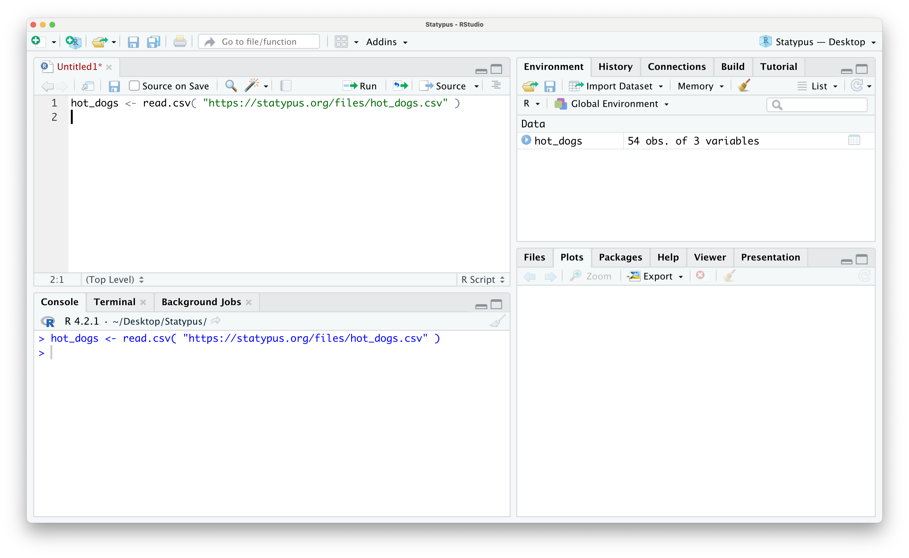
Figure 1.29: Looking at Data in the Environment
Use the str() function we have looked at above to see what kind of data are in the file.
You should see a new layout for the output of str() and this leads us to the topic of Section 1.3.4, Data Frames.
1.3.4 Data Frames
Definition 1.6 A Data Frame is a list of variables of the same number of rows. A data frame is thus a collection of different variables each of which is contained in its own column.
Example 1.16 In Example 1.15, we loaded the hot_dogs dataset and if you used str to look at it in the “Now it’s your turn!” after the example, you would have determined it was a data frame. To get a further look at hot_dogs, we will now run head on it as well.
##   type calories sodium
## 1 Beef      186    495
## 2 Beef      181    477
## 3 Beef      176    425
## 4 Beef      149    322
## 5 Beef      184    482
## 6 Beef      190    587
When we ran head on snickers, it returned the first 6 entries. Now head returns the first 6 entries of each of the 3 different variables contained in hot_dogs. To make the information above clear, we can interpret it that the hot dog listed in the first row was made of beef, contained 186 calories19, and also contained 495 milligrams of sodium.
To be clear, this is a single hot dog where we recorded 3 different data values for it. The first one was its “type” which is a character type variable. The other variables are numeric values called “calories” and “sodium”
Definition 1.7 While there are more nuanced ways of accessing information within a data frame, the dollar sign operator, $, is the easiest way to access values in a data frame.
If we have a data framed named df, then typing df$ into a script or into the Console should bring up a drop down menu of the variables contained in the data frame.
Example 1.17 Here we continue the work of Example 1.16 of investigating the hot_dogs dataset using the dollar sign operator, $. If you have hot_dogs in your Environment and type hot_dogs$ into a script or Console, you should see something similar to the following.
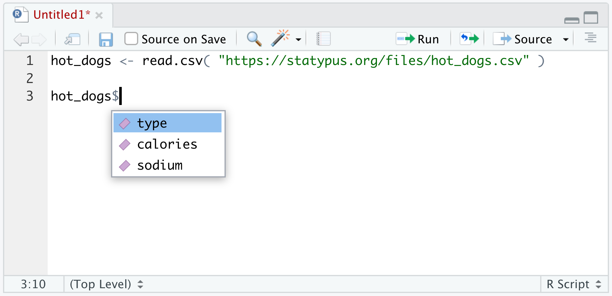
Figure 1.30: Using the dollar sign operator
Here we see that hot_dogs contains the 3 variables we mentioned in Example 1.16: type, calories, and sodium. If we click on (or use the keyboard arrow keys to select) sodium and run the line of code, we get the following.
##  [1] 495 477 425 322 482 587 370 322 479 375 330 300 386 401 645 440 317 319 298
## [20] 253 458 506 473 545 496 360 387 386 507 393 405 372 144 511 405 428 339 430
## [39] 375 396 383 387 542 359 357 528 513 426 513 358 581 588 522 545
This shows that hot_dogs$sodium is a vector of the amount of sodium in each of the hot dogs in the data frame. Similarly, we can look at the contents of the type variable using the following.
##  [1] "Beef"    "Beef"    "Beef"    "Beef"    "Beef"    "Beef"    "Beef"
##  [8] "Beef"    "Beef"    "Beef"    "Beef"    "Beef"    "Beef"    "Beef"
## [15] "Beef"    "Beef"    "Beef"    "Beef"    "Beef"    "Beef"    "Meat"
## [22] "Meat"    "Meat"    "Meat"    "Meat"    "Meat"    "Meat"    "Meat"
## [29] "Meat"    "Meat"    "Meat"    "Meat"    "Meat"    "Meat"    "Meat"
## [36] "Meat"    "Meat"    "Poultry" "Poultry" "Poultry" "Poultry" "Poultry"
## [43] "Poultry" "Poultry" "Poultry" "Poultry" "Poultry" "Poultry" "Poultry"
## [50] "Poultry" "Poultry" "Poultry" "Poultry" "Poultry"
This shows that we have 3 different values in the type: "Beef", "Meat", and "Poultry". Don’t forget that character strings should always be encased in quotation marks.
The dollar sign operator is a very useful tool for accessing values in a data frame, but there are more robust tools we can use. We can use the bracket operator, [ ], that we first used for vectors in Example 1.12 again for data frames to pull out subsets of the data frame. When we used the bracket operator for vectors, we only had to provide one input within the brackets. Now that we are using it for a data frame, we must pass it two different inputs. For discussion purposes, we will call these inputs R and C and they should be entered as df[ R, C] where df is the name of the data frame we are utilizing. The R input is what we will call the Row Rules and the C input is what we will call the Column Rules. Example 1.18 shows some examples of using these rules.
Example 1.18 (Accessing Subsets of Data Frames) To begin our investigation of how to use the bracket operator for data frames, we begin by loading a new data frame called BabyData1 which we will see numerous times throughout Statypus.
Use the following code to download BabyData1.
As suggested earlier, our first task is to run str() on the data set.
## 'data.frame':    200 obs. of  12 variables:
##  $ mom_age      : int  35 22 35 23 23 26 25 32 41 22 ...
##  $ dad_age      : int  35 21 42 NA 28 31 37 38 39 24 ...
##  $ mom_educ     : int  6 3 4 1 4 3 5 5 4 3 ...
##  $ mom_marital  : int  1 1 1 1 1 2 1 1 1 2 ...
##  $ numlive      : int  2 1 0 2 0 1 0 1 0 0 ...
##  $ dobmm        : int  2 3 6 8 9 10 7 12 11 2 ...
##  $ gestation    : int  39 42 39 40 42 39 38 38 36 40 ...
##  $ sex          : chr  "F" "F" "F" "F" ...
##  $ weight       : int  3175 3884 3030 3629 3481 3374 2693 4338 2834 2948 ...
##  $ prenatalstart: int  1 2 2 1 2 4 1 1 2 1 ...
##  $ orig_id      : int  1047483 1468100 2260016 3583052 795674 3544316 3726920 2606970 2481971 243759 ...
##  $ preemie      : logi  FALSE FALSE FALSE FALSE FALSE FALSE ...
This shows us that BabyData1 is indeed a data frame that contains information about 200 individuals and has 12 variables for each individual. Each individual (a term we will define in Chapter 2) in this data frame is a baby and we have 12 different data values for each baby.
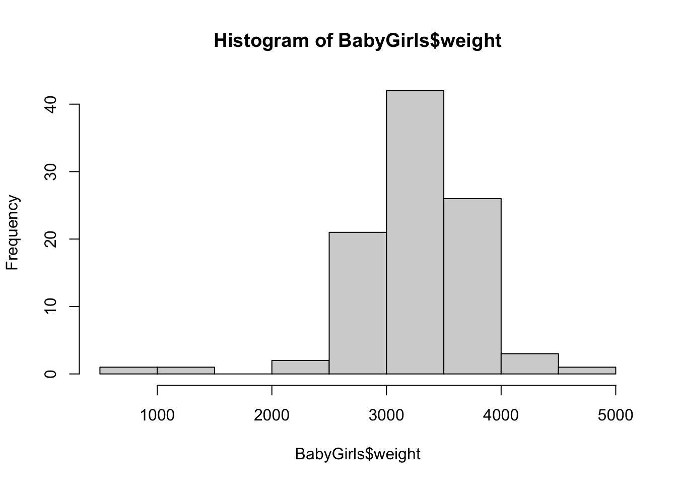
Let’s say we wanted to look at the distribution of the age of the mother of the babies. We could do this with the hist() function which we used in Example 1.6 and will fully explain in Chapter 3 along with the dollar sign operator.
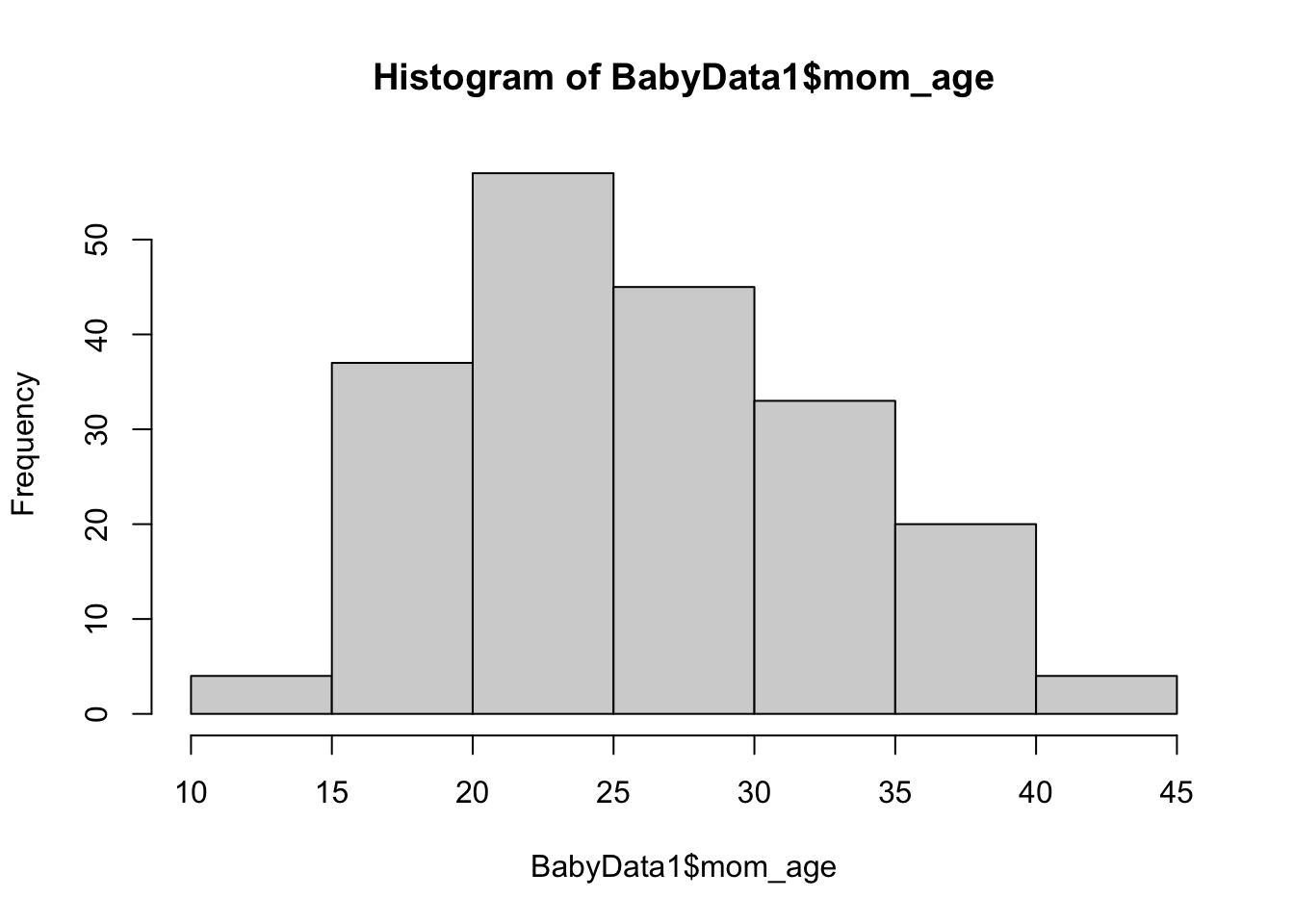 From here, we can glean a quick visual understanding of the ages of the babies.
The sex variable contains the sex of the baby. We can use the table() function which we will explain in Chapter 3 to see the contents of this variable.
##
##   F   M
##  97 103
This tells us that the 200 babies are comprised of 97 females labeled with an "F" and 103 males labeled with "M".
What if we were only curious about information about baby girls? For example, what if we wanted to look at the distribution of weights20 of only baby girls? We will attack this two ways.
Method 1: When we are working with a data frame for more than one inquiry
In this method, we will create a smaller data frame comprised of the rows of BabyData1 where we select only the rows where the sex variable is equal to "F". To do this, we set the Row Rule to be BabyData1$sex == "F" and leave the Column Rule blank so that we end up with all columns, but only the rows of values where the baby was female. We will save the result as a new data frame called BabyGirls.
The result is that R creates a new data frame of only the baby girls and stores it as BabyGirls as we can see in the screenshot below.
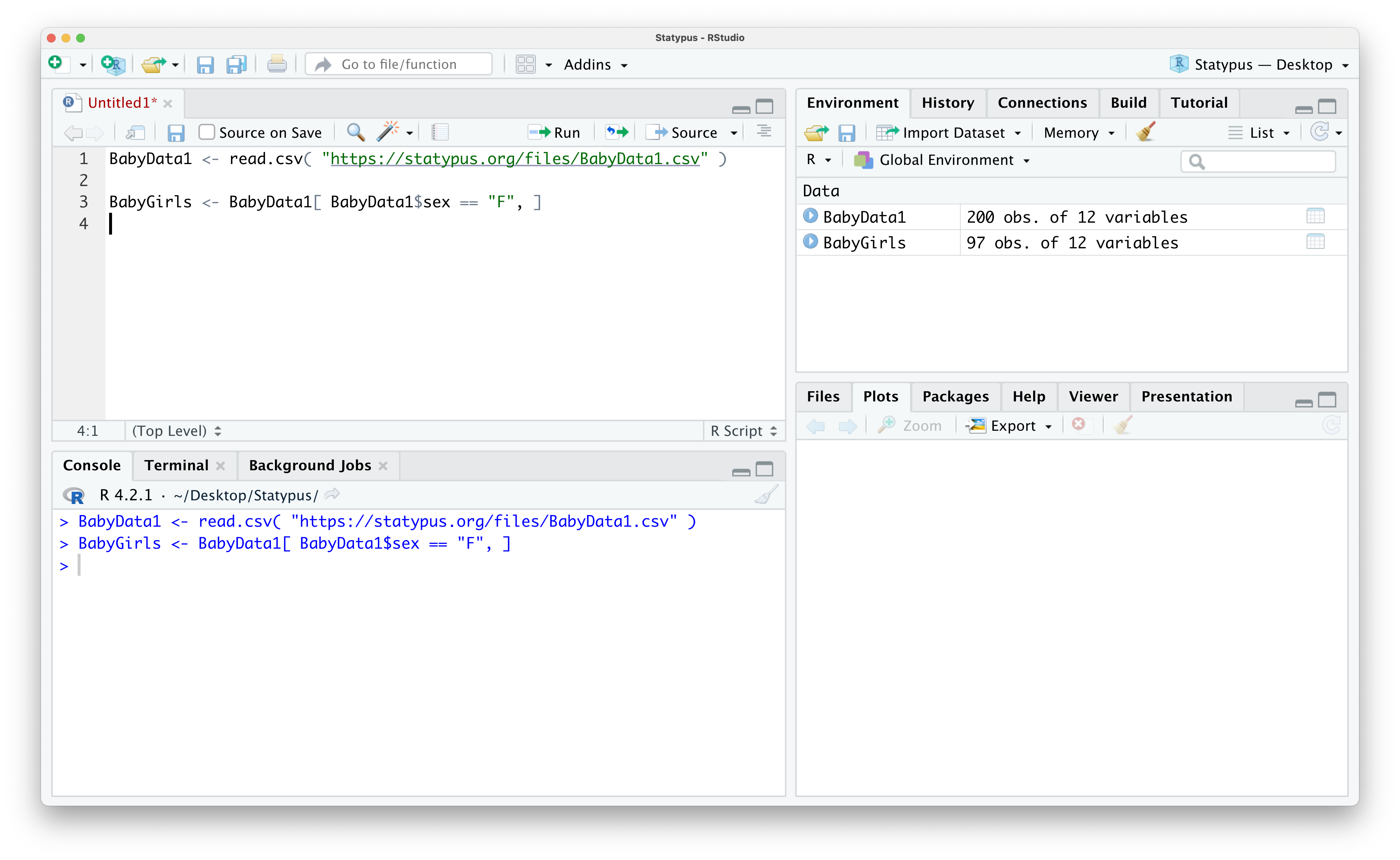
Figure 1.31: Creating a sub data frame
From here, we can simply use the dollar sign operator to create a histogram like we did for the full BabyData1 data frame.
Method 2: When we only need to do one thing with this data
In this method, we will first go into the data we want with the dollar sign operator and then use the bracket operator (now operating on a vector) to select the rule or restriction we have. To inch our way there, we begin by looking at the histogram of all baby weights.
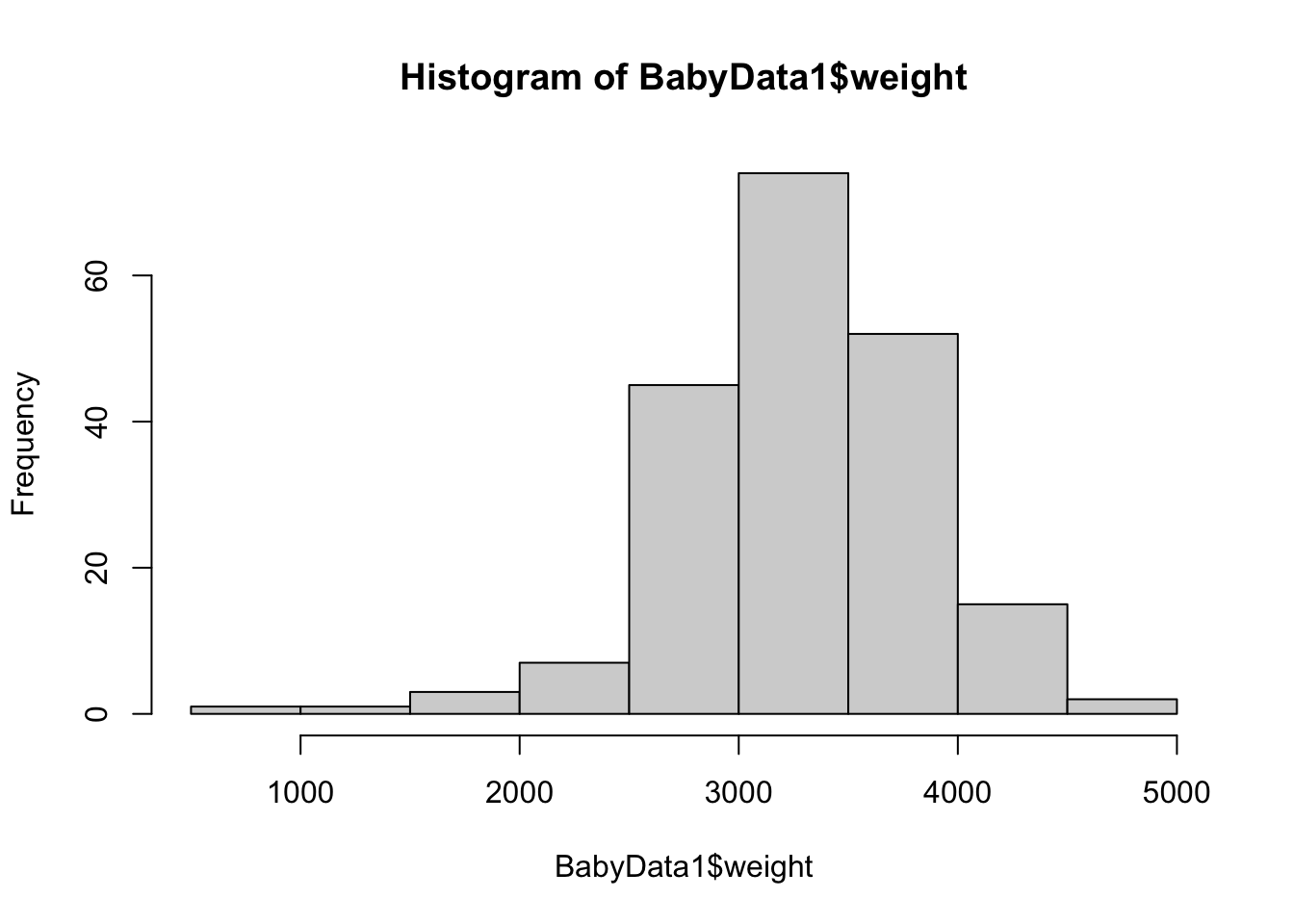 This is a great start, but it is the distribution of all babies, not just the females. To finish this, we will use the bracket operator to refine the vector we are making a histogram of.
Note that we only have a single input for the bracket operator now as once we used the dollar sign operator, we have a vector and not a data frame.
We will expand this discussion of using the dollar sign operator and bracket operator in Example 3.6.
1.3.5 Packages
One of the absolute strengths of R is the amount of “add-ons” that are available for it. While we will stick to what can be called “Base R Functions” here at Statypus, there is an incredible amount of functions which can easily be added via Packages. A Package is a collection of data, new functions, and the necessary associated documentation for it all saved and distributed in a way to make it easily accessible to all R users. Packages such as dplyr have allowed users a much easier “grammar” when doing “data wrangling”21 while packages such as ggplot2 have added amazing new tools for data visualizations. Other packages such as knitr and bookdown can be used to create simple statistical reports or resources as complex as this textbook!
There is no denying that the power of R is greatly expanded when one uses certain packages, but here at Statypus, we will use as few packages as possible to focus on code that will work regardless of what packages are currently loaded. The mentality is that we want our code to work on a “fresh install” of R without the need to call on packages before running our code. All of the skills learned here will easily translate to the use of more advanced packages that may be required for the specific analysis being done by a particular researcher.
As an example of how to install a package, we will show the steps to install theHistData package. To do this, look in the lower right pane and select the “Packages” tab. The pane should now look like the one below.
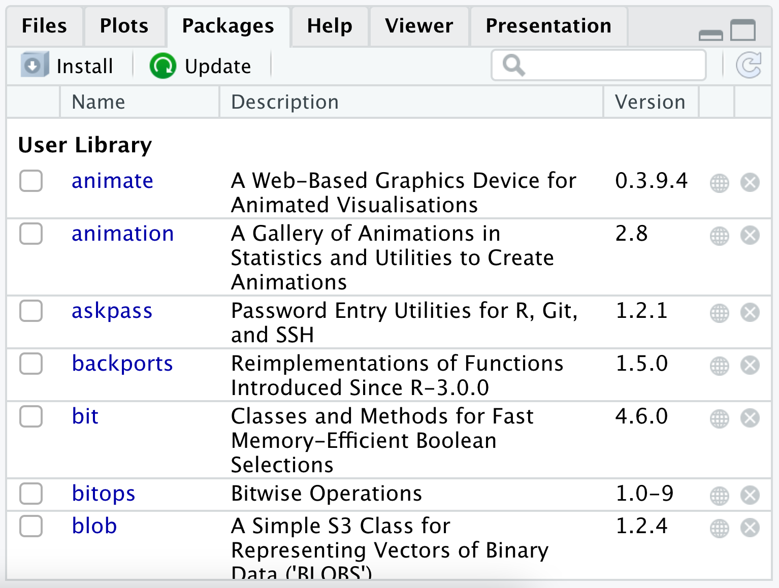
Figure 1.32: Using the Packages tab
From here, you can begin typing in HistData into the search bar (the one with the magnifying glass) without concern of being case sensitive. Once you have typed in hist you will see only the package we are interested in, HistData. Clicking the checkbox to the left of HistData will automatically load the package onto your machine as shown below.
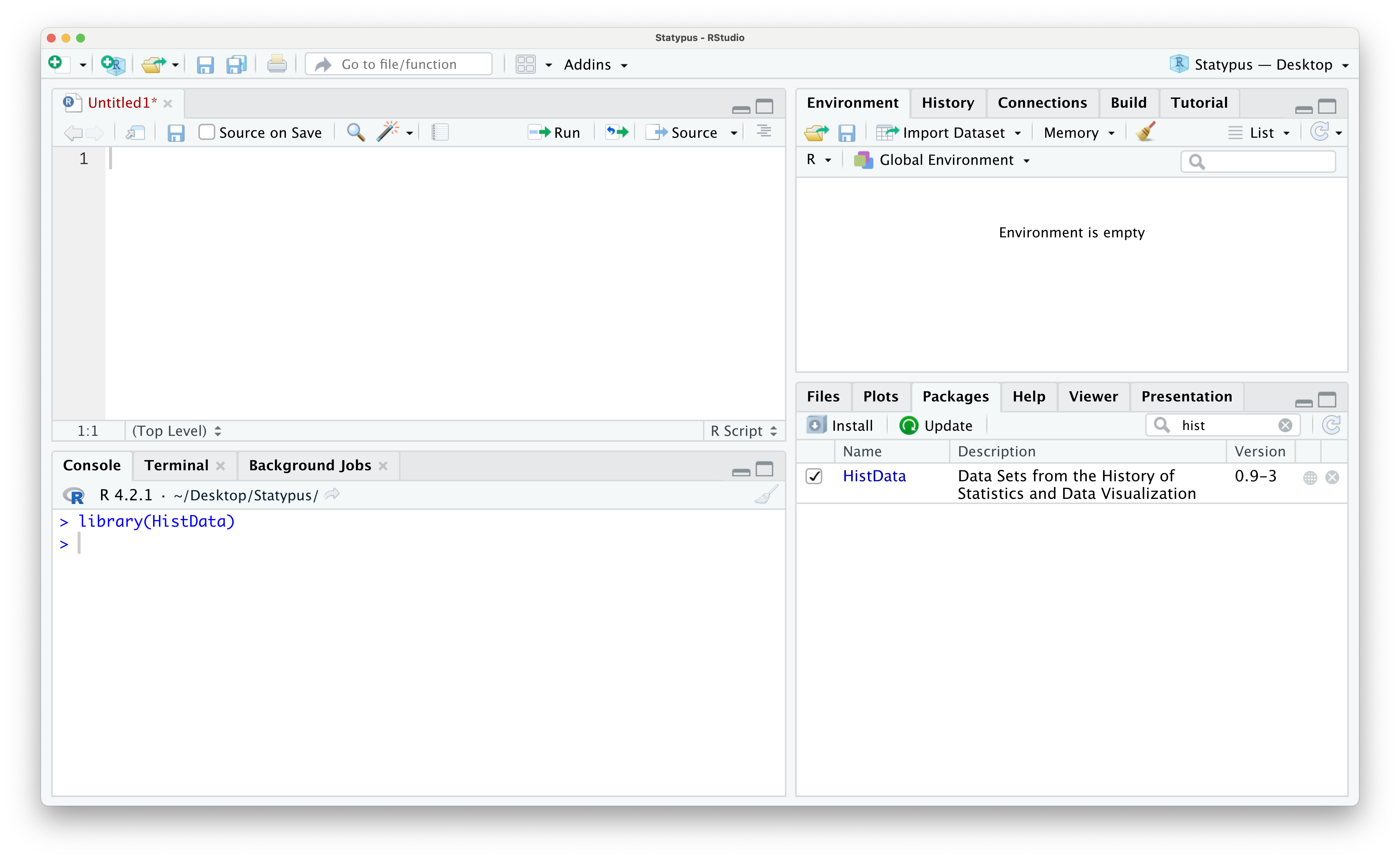
Figure 1.33: Using the Packages tab
Once you have loaded HistData you have access to all of the files contained in it. For example, we can access the DrinkWages data frame as shown below.
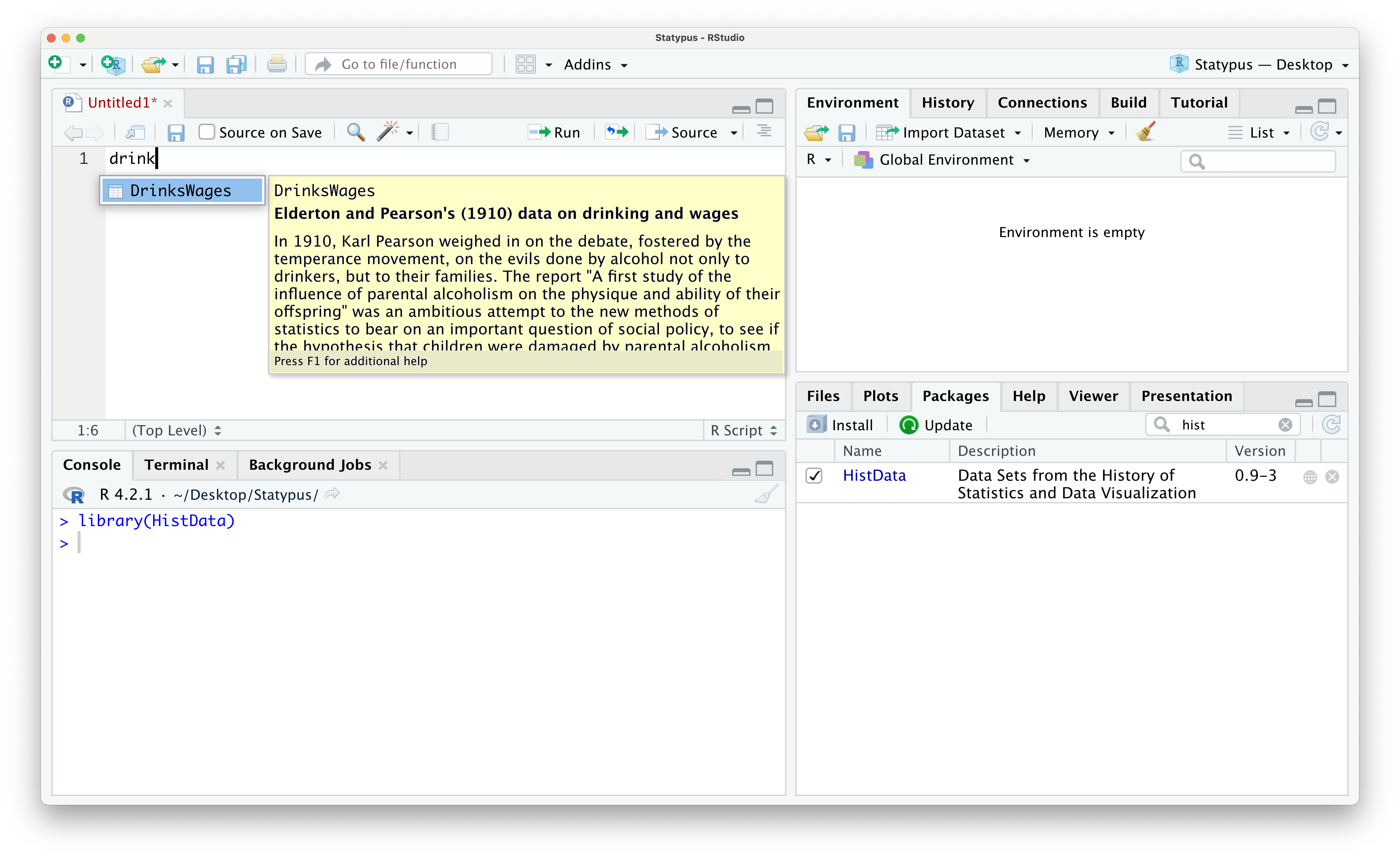
Figure 1.34: Using the Packages tab
1.4 Functions
R is a functional programming language. While we will not get anywhere near the depths that one can go with this concept here at Statypus, the takeaway is clear: our primary way of utilizing the power of R is through the use of functions.
In Example 1.9 we ran the following line of code: sort( snickers, decreasing = TRUE ). This is an example of running an R function and shows the basic syntax we will use, which is shown below.
functionName( argument1, argument2, argument3 )In R, functions can have more than one input (called arguments), we show 3 above, but it can be more. Moreover, those arguments can at times be long to type out so that the above syntax may stretch well across your computer screen. If we wanted to make the code a little easier to read, we could rewrite the above syntax as follows:
functionName( argument1,
argument2,
argument3 )When looking at the above, when R gets to the first parenthesis, (, it knows to begin looking for arguments for functionName and it continues to do so until it hits the closing parenthesis, ). Regardless of how you type it out on the screen, you should have a comma after each argument except for the last one which should be followed by ).
Example 1.19 Here is a chunk of code that will find correlation (which we will define in Chapter 5) between the age of a baby’s mother and the age of its father using a dataset we imported in Example 1.18.
## [1] 0.7516507Here the 3 arguments that we pass to cor are x, y, and use.
We will see why we invoked the use argument in Section 1.5.6 and in more detail in Chapter 5.
The above code may not run if you copy and paste it into your computer. To make it run, you would first need to import the BabyData1 like we did in Example 1.18.
Functions can also have more than one output. This may go against the definition of a function that you learned, but the most important concept is still true. The output of a function is uniquely determined by the arguments that we pass to the function.22
We can see what arguments a function wants by typing in the function, such as sort(), into an R script (or in the Console) and waiting. A yellow pop-up will appear showing the arguments that the function needs passed to it.
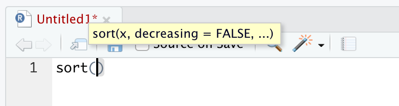
Figure 1.35: The pop-up showing the arguments of sort()
This shows that the main arguments are x, the data to be sorted, and decreasing which is set to FALSE by default as indicated in the pop-up. The ellipsis indicates that there are other, and lesser used, arguments which we can look at by using the help option by running ?sort.
1.5 Help, Warnings, and Errors
Like we said in the Preface, it is our firm belief at Statypus that we learn by making mistakes. It is inevitable that you will encounter mistakes if you engage with R or any software. Mistakes when working with computers can come in many different forms as we will see in this section.
A lot of mistakes can be avoided if the user starts a new “session” of RStudio each time they interact with it. To do this, make sure to do the following steps each time you are done working in RStudio.
1. Save any open R script.
For example, the following screenshot shows us working with the “GoldenRatio.R” R script we built in Example 1.3 and if you look in the tabs of the upper left pane, you will see that “GoldenRatio.R” is displayed in red indicating that it needs saved. You should save it by using the “Save current document” icon (it resembles a computer diskette) which appears directly below the .R of “GoldenRatio.R” below.
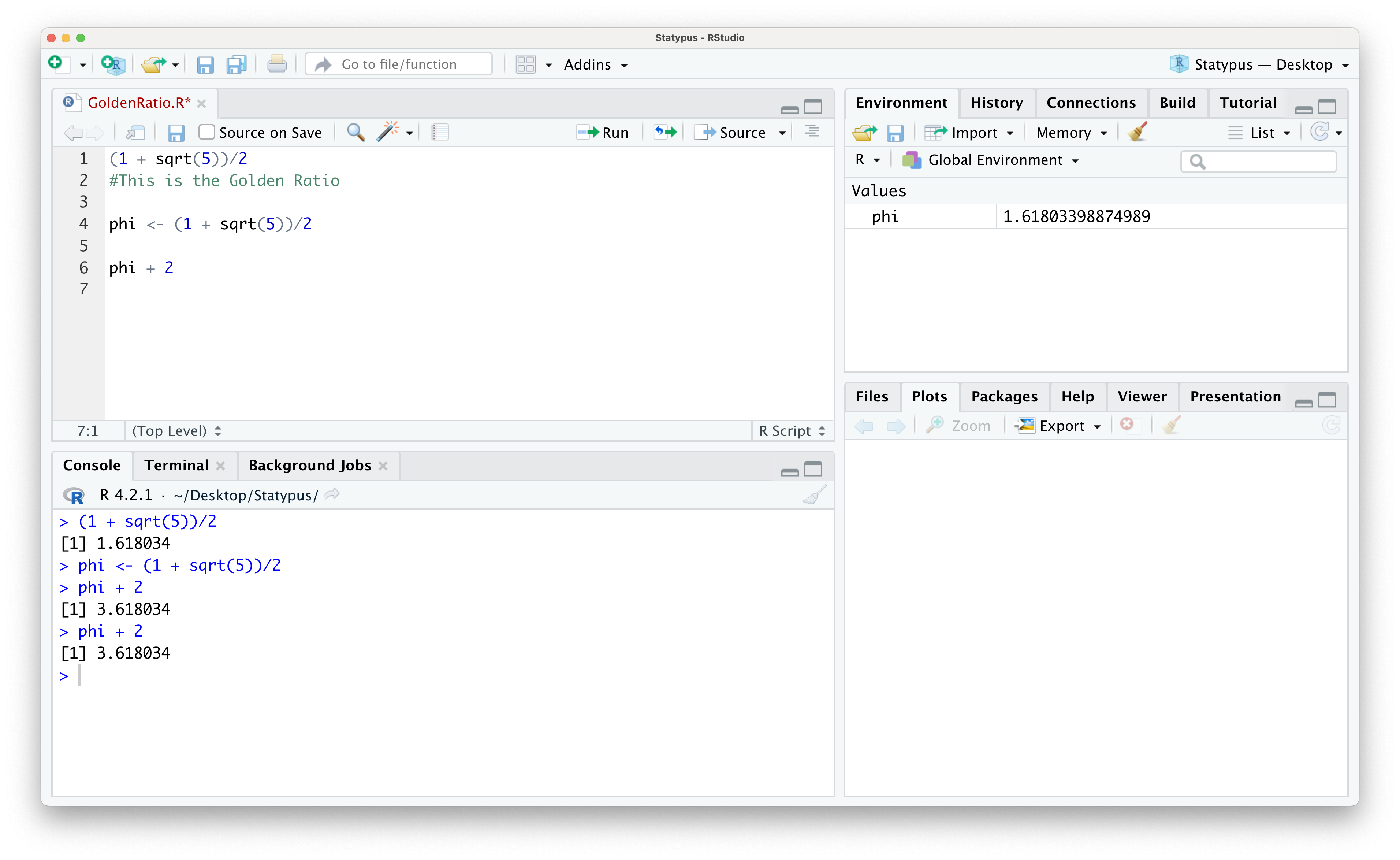
Figure 1.36: Saving an R Script
2. Shut down RStudio
Once you have saved all of your open documents, it is time to shut down RStudio. When you do so, you should see a dialog box like the following appear.
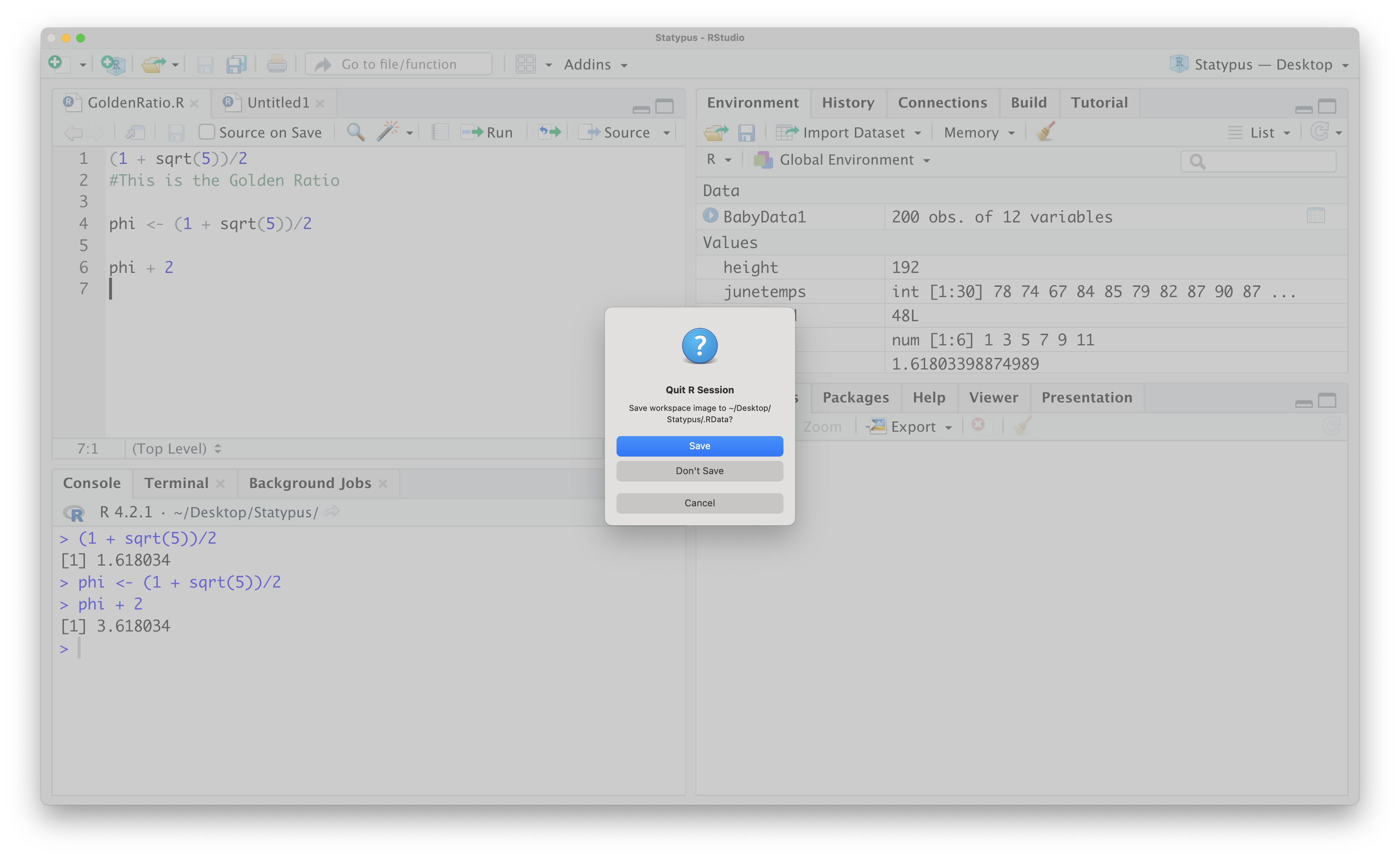
Figure 1.37: RStudio Shutdown Dialog Box
At this point, we come to the most important step.
3. Make certain to select Don't Save on the dialog box shown above.
1.5.1 Built-in Help
Before looking at the types of mistakes we can make, we begin by looking at how R offers help in order to avoid or “debug” them. Every dataset or function built into R has a Help page which will appear in the lower left pane of RStudio. This is most easily accessed using the Question Mark Operator or ? which we demonstrate in Example 1.20.
Definition 1.8 The Question Mark Operator or ? is a shorthand for the more formal help() function.23 It is the primary interface to the help systems.
Example 1.20 In Example 1.9, we used the sort()function but didn’t give any information on what exactly this function did. To see the help file R has built in, we simply run the command ?sort (or ?sort()) in either a script or the Console.
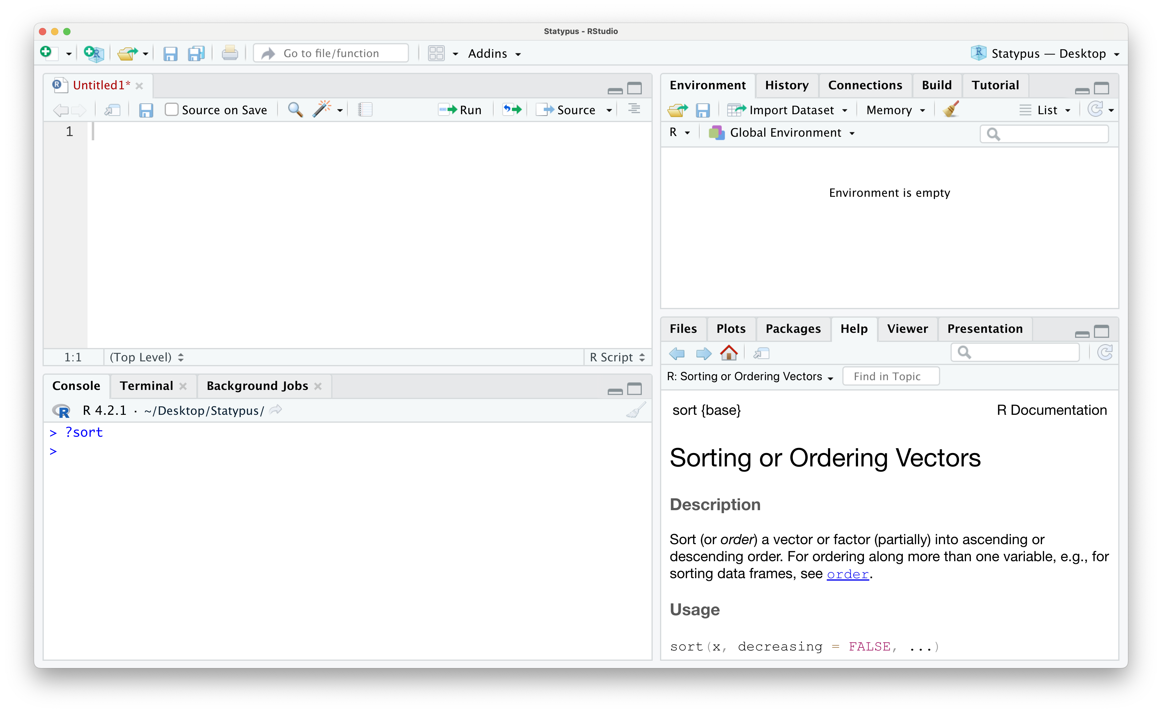
Figure 1.38: The help file of sort()
In Section 1.2.1 we saw the rivers dataset in Example 1.4. This dataset also has built in help which can be accessed using the following line of code.
The result of running this line of code is shown below.
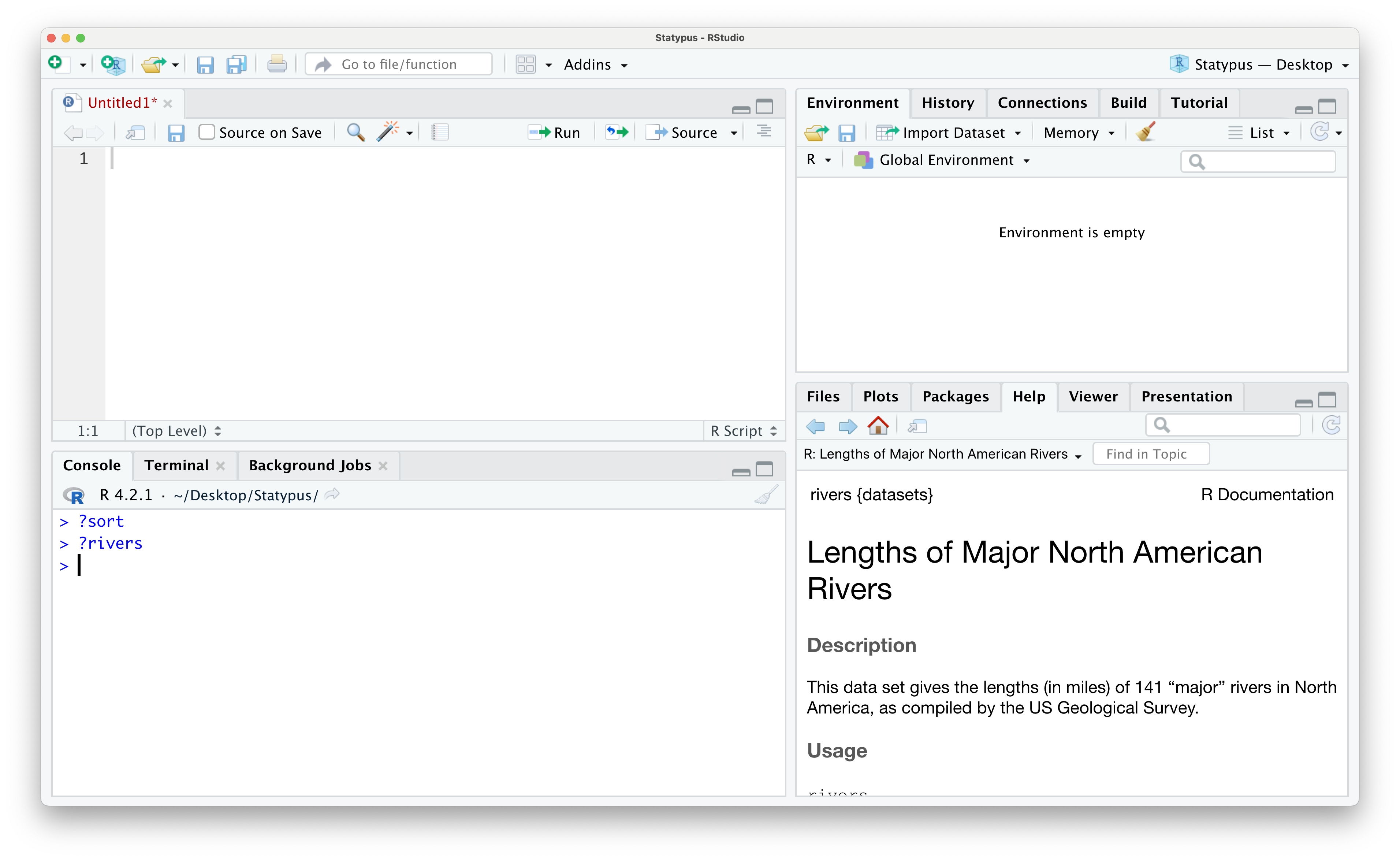
Figure 1.39: The help file of rivers
One of the benefits of loading data and functions from packages is that they are required to have help files which can be accessed with the question mark operator. For example, if you installed the HistData package like we discussed in Section 1.3.5, you could find more info about the DrinkWages data frame by running ?DrinkWages in either a script or the Console.
1.5.2 Typos
Unfortunately, despite our best efforts, we can simply make typographical errors or typos. This is a major reason why we offer code on Statypus that is easily copied to your machine’s clipboard. However, typos are still inevitable.
At Statypus, we highly encourage the Type Three Rule. That is, you should type the first three characters of the element you are looking for and then using the menu to select the appropriate value.
If you begin typing (at least the first three characters of) something into RStudio, auto-complete will search for all things in memory, data or functions, in a non-case-sensitive way and allow you to choose from a drop down list. For example, typing vie into an R script or into the R console it will pop up a menu to allow you to choose the function, View(), as shown below.
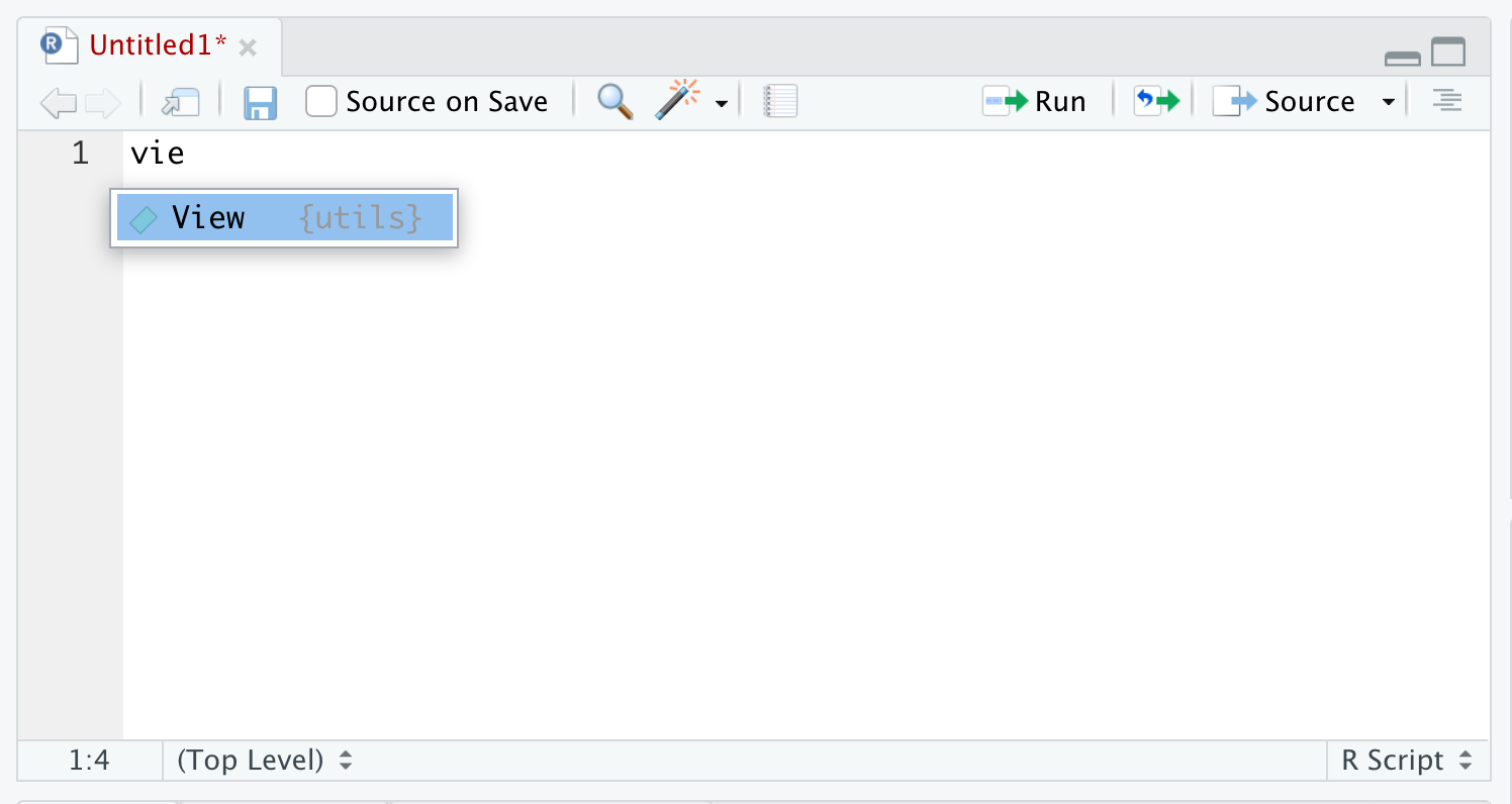
Figure 1.40: Autocomplete Example
If there are more than one option for the three characters for what you type, you get a dropdown menu showing all of the objects that begin with that regardless of case. For example, below is what you will likely see if you type in bar into R.
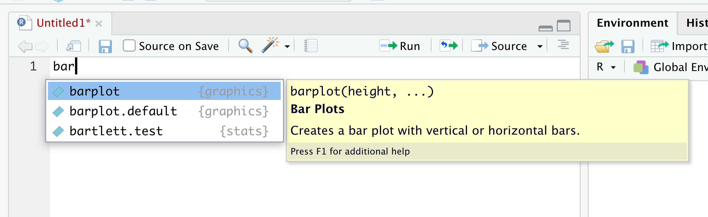
Figure 1.41: Autocomplete Example
From here, you can choose the function you, maybe the function barplot() which we will introduce in Chapter 3.
Many typos can be avoided by following the Rule of Type Three as R is case-sensitive so that view( snickers ) causes an error while View( snickers ) will display the vector snickers in the upper left pane of RStudio (assuming it has been loaded like we did in Example 1.9).
## Error in `view()`:
## ! could not find function "view"
1.5.3 Errors
As we saw in the Remark at the end of Section 1.5.2, errors are inevitable. Computers are amazing tools, but they do require very precise input to operate correctly. Beyond just spelling things correctly as we saw in Section 1.5.2, you must also use the correct syntax. When R encounters an Error, it has encountered a problem which makes it unable to complete the task asked of it. It will display an Error in the Console and we will see examples of this below.
Example 1.21 As we mentioned in Example 1.8, character strings should always be contained in quotation marks. In that example we ran the line of code below to store the character string "AB" into the variable bloodType.
However, a very common mistake for beginners to make is to forget to include the quotation marks like show below.
## Error:
## ! object 'AB' not found
Because there are no quotation marks around AB above, R attempts to find an object (existing data or function) that is named AB. Since there does not exist an R object named AB, RStudio simply reports that no such object was found.
Users new to working with computer software that requires them to enter code into a terminal manually like we do with R may be a bit confused about the distinction between parentheses, ( ), and brackets, [ ]. In most students’ experience, these grouping symbols have been used interchangeably in their previous math coursework. However, R is very particular about every symbol that the user offers it. It is possible that students would be quite comfortable with the expression \(f(x)\), but may be perplexed if they saw it written as \(f[x]\). This will be our mental trick to remembering when to use parentheses. We will always use parentheses following a function.
Example 1.22 As as example, earlier in Section 1.2.1, we saw the square root function which was utilized via sqrt(). Attempting to use brackets will yield the following Error:
## Error in `sqrt[16]`:
## ! object of type 'builtin' is not subsettable
Because we followed sqrt with the bracket operator, R thinks we are looking for a subset or portion of a data object. Since sqrt is a function and not data, RStudio is letting us know it cannot use the bracket operator to pull out a subset of it.
The bracket operator is used to access certain parts of vectors and data frames called subsets. Attempting to use parentheses when you should be using the bracket operator will cause an error as shown in Example 1.23
Example 1.23 Similarly, if we used parentheses when we should be using the bracket operator, we get a similar type of error. If we had the vector snickers in our Environment and tried to access the first entry with the following line of code it give an error.
## Error in `snickers()`:
## ! could not find function "snickers"
Here, since we followed an object with parentheses, it assumes that we are trying to call a function called snickers. Like we saw in Example 1.21, that object doesn’t exist because snickers was a vector.
Examples 1.22 and 1.8 give a validation of why it is imperative to name objects wisely. Having both a dataset and function saved with the same name can cause immense difficulty at times which is why we suggested not using names like sum or mean for data values in Section @(basicdatatypes).
We have seen that the two sets of grouping symbols, ( ) and [ ], serve very different purposes and must be kept straight by the user.
Parentheses
The parentheses can be used as as typical grouping symbols when making calculations such as when we calculated the Golden Ratio in Example 1.5 with the following line of code.
As we saw in Section @(), we also use parentheses to hold the arguments we want to pass to a function like the “mock” code shown below.
functionName( argument1 )Brackets
The bracket operator, however, should not follow a function, but a piece of data such as a vector or data frame.
For vectors, we use a single logical rule as shown in the “mock” code below.
vector[ Rule ]For data frames, we use two different logical rules as shown below in “mock” code.
df[ R, C ]Here R is rule applied to the rows and C is the rule applied to columns. As we will see in Example 3.6, a rule can be made up of more than one logical test if we combine them with the Logical And Operator, &, or the Logical Or Operator, |.
There is also a third set of grouping symbols, braces or { }, which are used to group lines or code to be ran at once. We won’t introduce these until Chapter 13 when we look at simulations. Attempting to use braces where parentheses or brackets will likely also give a Warning or an Error.
Additionally, there are other and more advanced uses of parentheses and brackets. For example, parentheses are used when doing certain logical conditionals such as if or when. These are concepts we will not cover in this book, but the techniques can be invoked by advanced users. For brackets, there is also a double bracket operator which performs a similar operation as the bracket operator we have looked at, but does do things slightly different. The super curious reader can see forums such as Stack Overlow to dive deeper.
Example 1.24 One of the most frustrating errors that beginners often encounter occurs when they have run completely correct code. In Example 1.6 we made our first plot where we constructed a histogram of the rivers vector which was produced as Figure 1.23. However, below is a screenshot of an RStudio session just prior to running the line of code hist( rivers ).
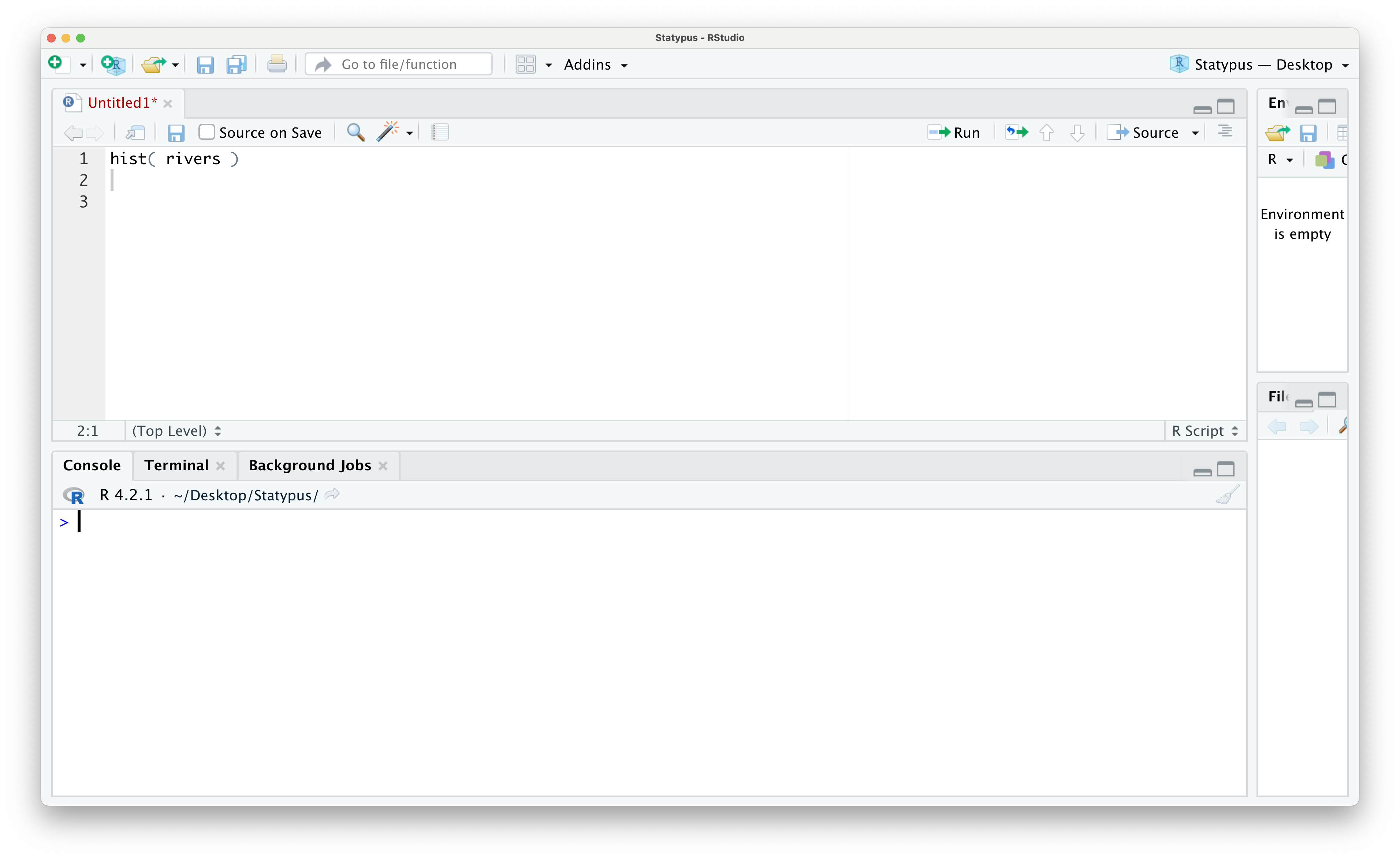
Figure 1.42: Our First Plot Error
however, if we run this code now, we see the following appear in the Console.
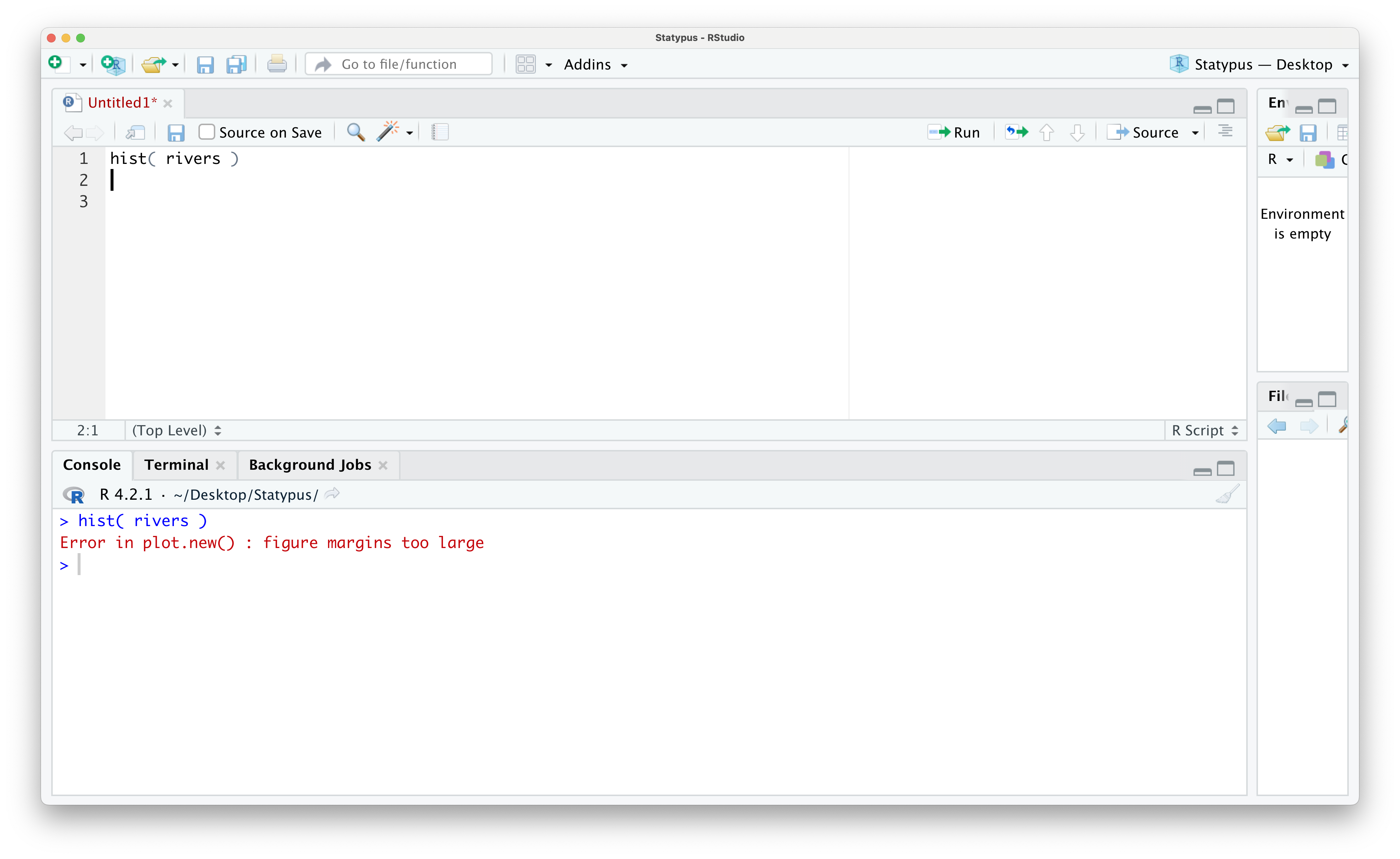
Figure 1.43: Our First Plot Error
The error message of Error in plot.new() : figure margins too large displays very prominently and convinces many beginners they have done something significantly wrong. However, all this error is telling the user is that RStudio was unable to display the plot that was requested because the size of the lower right pane was too small to draw it. In a very literal sense, R simply says it needs more paper to draw the plot.
This is a fairly common error as users will often find it easier to expand the size of the left panes to make their interaction with RStudio easier to see. However, this is often done at the expense of making the right panes too small to serve their purposes. If you place your mouse over the vertical divider of the left and right panes, a little “left-right arrow” cursor should appear. You can now “grab” this vertical divider and drag it towards the let allowing the lower right pane to have enough room to display our plot.
Unfortunately, RStudio will not automatically just retry to make your plot, but you need only move your cursor back to your code and rerun the line that failed as shown below.
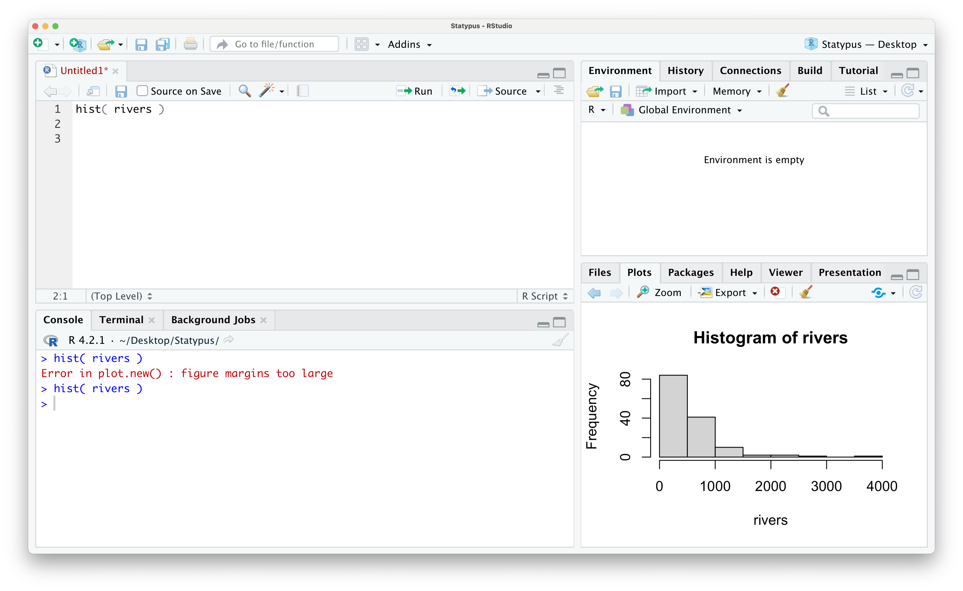
Figure 1.44: Our First Plot Fixed
Example 1.25 We conclude this section with one of the most classic Errors for R users. It is fairly customary to create a working copy of a data frame and give it a short and easy name, such as df. We show the process of this at the end of Section 1.5.6.
There we created a copy of the data frame BabyData1 and called it df and were able to extract data from it using the command df$sex. However, if we reloaded a script with this command and had not yet created the working copy, df, then we would get the following Error.
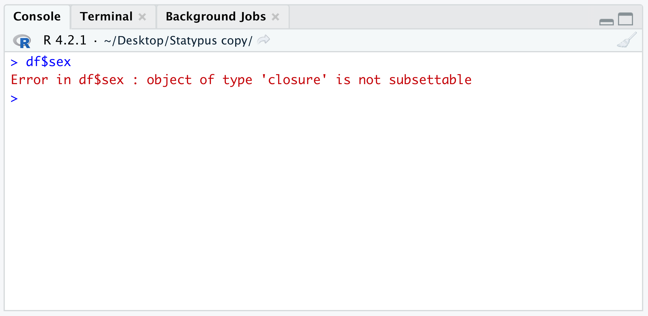
Figure 1.45: The Classic df Error
The result here is very similar to what we encountered in Example 1.22 where we attempted to use brackets on a function. You may have expected a result more like the Error found in Example 1.21 where an object was not found. However, the hidden fact you may not know is that df is actually a built in function dealing with something called the “F Distribution.”
1.5.4 Warnings
While errors left R unable to complete the task that it was trying to do, R can also encounter issues it is able to remedy in certain ways. When R encounters issues it is able to overcome to a level to produce a result, it will provide the user with a Warning in the Console as it produces the result. We will look at a few examples now.
Example 1.26 We will deal with missing data more in Section 1.5.5, but missing values can be one of the most common causes of Warnings. For example, in the following block of code we create a vector of values of the values 1 through 4, but where for some unknown reason, the value of 3 was reported as missing.
If we look at the structure of x using str() we see that it is saved as character strings.
## chr [1:4] "1" "2" "missing_value" "4"The as.numeric() function attempts to convert numbers saved in character strings to their numeric equivalent. As a quick example we see the following.
## [1] 7However, if we apply as.numeric() to x, we will obtain a Warning.
## Warning: NAs introduced by coercion## [1] 1 2 NA 4This shows that as.numeric() returns both an NA character (which we will fully discuss in Section 1.5.5), but also returns a Warning. We show what this looks like within RStudio below.
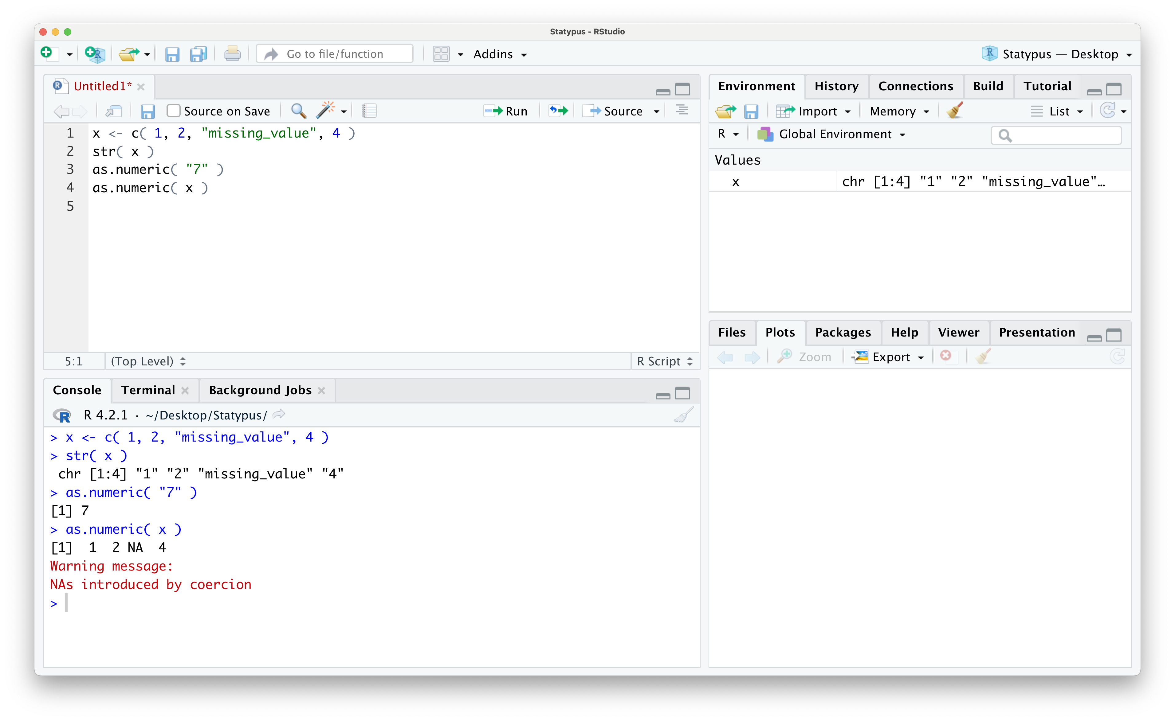
Figure 1.46: Our First Warning
The as.numeric() introduces an NA character for each string which is not numeric (when removing the quotation marks). While you may never use the as.numeric() function directly, it is possible for a similar error to appear as certain functions will try to convert character strings to numeric data in order to make calculations.
Example 1.27 In Example 1.13 we looked at some of the basic vector arithmetic we could do involving the vectors below.
However, we never attempted to simply add x and y. Doing so yields the following Warning.
## Warning in x + y: longer object length is not a multiple of shorter object
## length
## [1] 4 6 6The result is the vector 4 6 6 which is result of adding the first component of x to y and then the corresponding second components, but the third component is where things get tricky. As x only has 2 entries, R decides to “start over” and use the first entry of x with the next (third) entry of y giving 6 in the third position of the result.
The Warning that R gives us is really that it didn’t finish using x once it started using it again. For example if we define a new vector, w, which has 4 entries, we can successfully add x to w and it offers no Warning. Here R used x a full two times adding the 2 entries of x to the first 2 entries of w and then to the third and fourth entry.
## [1] 7 9 9 11Here R used x a full two times adding the 2 entries of x to the first 2 entries of w and then to the third and fourth entry. This also works with multiplication like we show below where again we have no Warning since x twice when multiplying entries of w.
## [1] 6 14 8 18Example 1.28 In Section 1.3.5, we saw how to load packages using both the Packages tab. However, we could have also used the install.packages() function. For example, the following line of code will also load the HistData package:
However, we really encourage using the Packages tab as simply misspelling the name of the packages leads to a very common and confusing warning. Below shows an attempt to install the BSDA package (which we introduce in Section 10.5.3) where we mistakenly use all lower case letters.
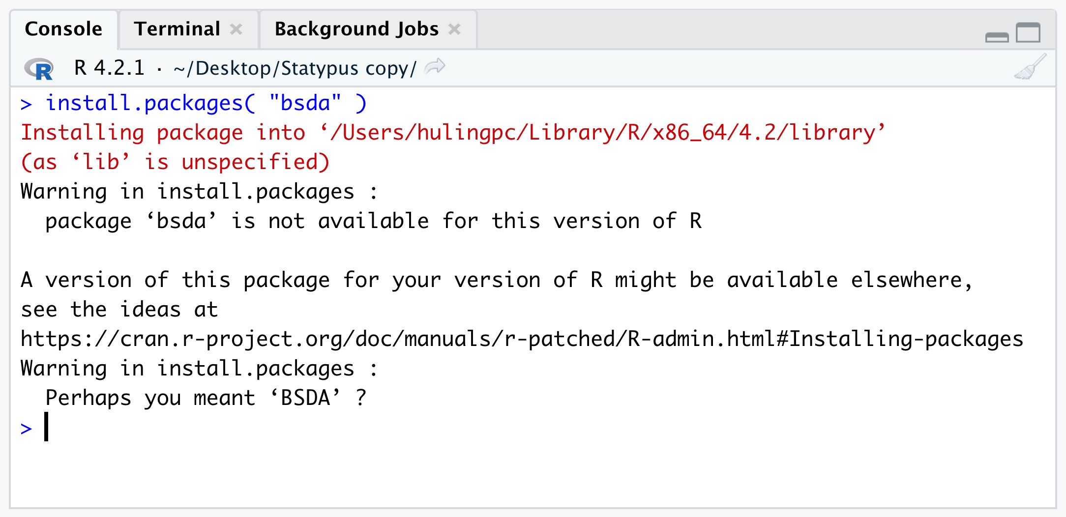
Figure 1.47: Mispelling a Package Name
Some users interpret that their version of R is out of date and that they need to update their computers. However, all the Warning is telling us is that it could not find any Package of name bsda when it looked in the CRAN repositories. This is because bsda doesn’t exist, but BSDA does. Searching for bsda in the Packages tab would alleviate this as shown below.
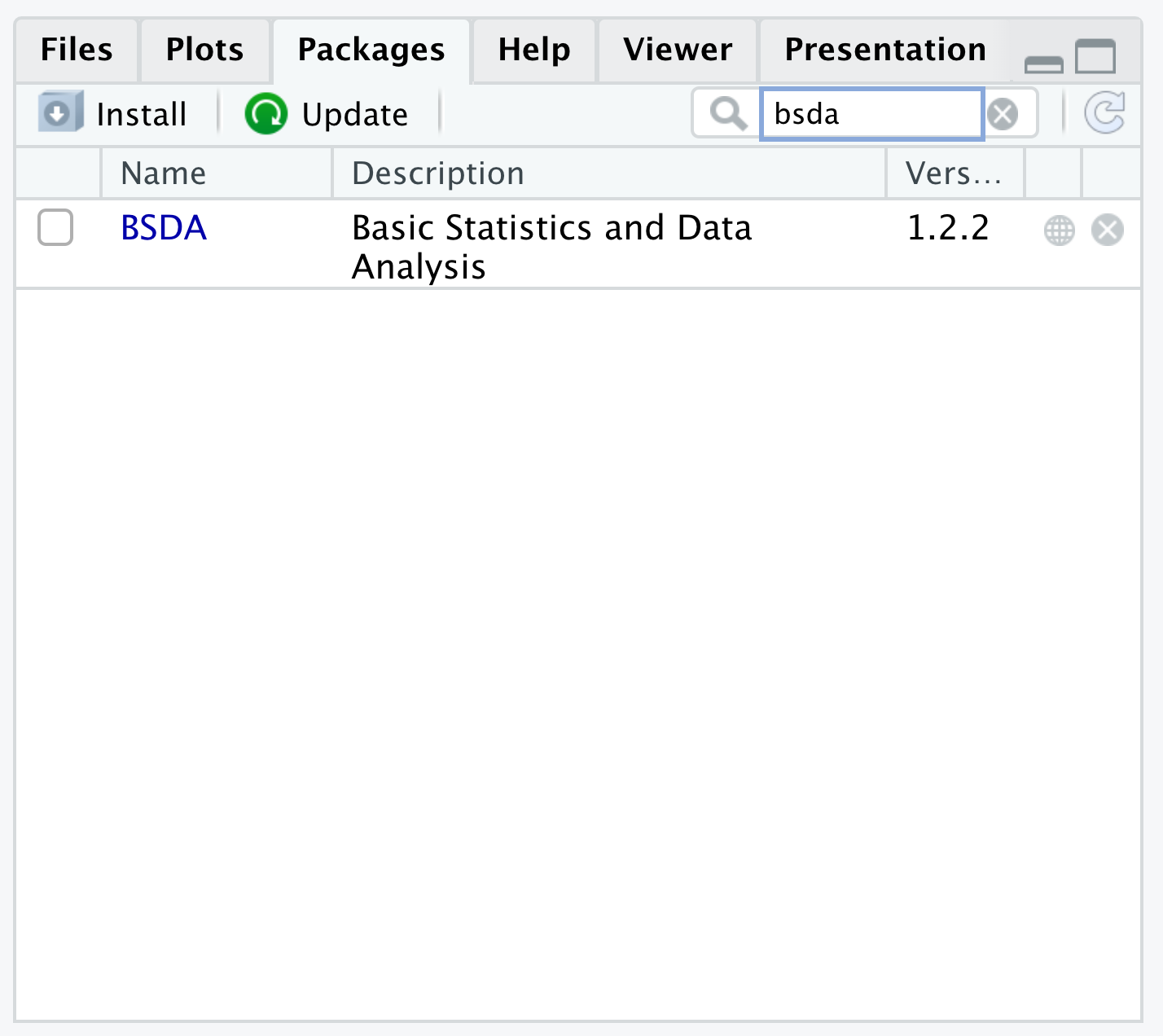
Figure 1.48: Mispelling a Package Name
1.5.5 Missing Data
Despite the best efforts of researchers, it is inevitable that some values of data may be missing from a dataset. Maybe a sensor didn’t malfunctioned and didn’t record a value or an individual left information off of a survey they were filling out. Regardless of the reason, it’s just a matter of reality that some data will be missing in most “real” datasets. The characters NA24 are used by R to indicate a single instance of where data should be, but where there is no value in the dataset. Below we see a typical result of what can happen if you have missing data.
Example 1.29 In Example 1.19, we ran the following chunk of code to find the correlation between the age of a baby’s mother and the age of that baby’s father.
## [1] 0.7516507The curious reader may have wondered why we used the argument use = "complete.obs". To see why, let’s see what happens if we simply omit it.
## [1] NAWhat is R trying to tell us? To understand this, let’s look at the first few values of the BabyData1#dad_age vector using head().
## [1] 35 21 42 NA 28 31Here we see that the fourth entry is also the curious NA we saw a second ago. According to R, “NA is a logical constant of length 1 which contains a missing value indicator.” To put this in simpler terms, NA indicates a single instance of missing data. For whatever reason, the age of the fourth baby was not recorded.
In a loose sense, this means that the age of the fourth dad could be thought of as “I don’t know.” We could use the following line of code to add the third and fourth values of BabyData1$dad_age.
## [1] NAIf someone asked you what the value of 42 plus “I don’t know” is, you would likely respond “I don’t know” or NA.
As we saw in Example 1.29, missing values can cause surprising results from functions. The correct way to handle missing values varies by the function which we will discuss in the coming chapters.
In general, however, a result of NA is simply R’s way of telling us that some data value is missing and it is up to us as the user to decide if we want to take further measures to get a different result.
1.5.6 Corrupted Data
Outside of causing Errors and Warnings, users can actually corrupt or “mess up” the data they are working with. This occurs unexpectedly frequently with beginning users as seemingly innocent lines of code can change or remove data. Even advanced coders can end up with undesired changes to their code due to very simple syntactical mistakes.
Example 1.30 In Example 1.18 we saw how to extract information about a subset of a data frame. In that example we ran the following line of code and got the subsequent result.
We did this based on the structure we first used in Example 1.12 and the Big Idea that followed it. That is, we indexed the vector BabyData1$weight by the logical vector that resulted from BabyData1$sex == "F" which tested if the value of the variable sex was "F" and gave a TRUE if so and a FALSE if not. Combining the two left us with only the values of the weight variable for babies that were female.
However, what if we made the seemingly innocent mistake of only using a single equal sign like below?
Well if we run the line of code, nothing appears to happen. But… if we were to then look at the data frame again, we would notice something has changed. In particular, here are the values of the sex variable found using the dollar sign operator.
##   [1] "F" "F" "F" "F" "F" "F" "F" "F" "F" "F" "F" "F" "F" "F" "F" "F" "F" "F"
##  [19] "F" "F" "F" "F" "F" "F" "F" "F" "F" "F" "F" "F" "F" "F" "F" "F" "F" "F"
##  [37] "F" "F" "F" "F" "F" "F" "F" "F" "F" "F" "F" "F" "F" "F" "F" "F" "F" "F"
##  [55] "F" "F" "F" "F" "F" "F" "F" "F" "F" "F" "F" "F" "F" "F" "F" "F" "F" "F"
##  [73] "F" "F" "F" "F" "F" "F" "F" "F" "F" "F" "F" "F" "F" "F" "F" "F" "F" "F"
##  [91] "F" "F" "F" "F" "F" "F" "F" "F" "F" "F" "F" "F" "F" "F" "F" "F" "F" "F"
## [109] "F" "F" "F" "F" "F" "F" "F" "F" "F" "F" "F" "F" "F" "F" "F" "F" "F" "F"
## [127] "F" "F" "F" "F" "F" "F" "F" "F" "F" "F" "F" "F" "F" "F" "F" "F" "F" "F"
## [145] "F" "F" "F" "F" "F" "F" "F" "F" "F" "F" "F" "F" "F" "F" "F" "F" "F" "F"
## [163] "F" "F" "F" "F" "F" "F" "F" "F" "F" "F" "F" "F" "F" "F" "F" "F" "F" "F"
## [181] "F" "F" "F" "F" "F" "F" "F" "F" "F" "F" "F" "F" "F" "F" "F" "F" "F" "F"
## [199] "F" "F"
Because of our use of only a single equal sign, we used the Equal Sign Assignment Operator and not the Equal Sign Test Operator and have assigned the value of "F" to ever single slot of BabyData1$sex.
Unfortunately, some steps in R (or any programming language) cannot be easily undone.25 However, with a bit of patience, we can recover from this mistake. The simplest solution is to simply remove the data frame and reload it. To do this, we first call on the remove function, rm().
We have successfully removed BabyData1 which we can verify by trying to run the following code.
## Error:
## ! object 'BabyData1' not found
We now simply reload BabyData1 using the line of code we got from Example 1.18.
To ensure that we have “fixed” our mistake, we again look at the sex variable.
##   [1] "F" "F" "F" "F" "F" "M" "F" "M" "M" "M" "F" "F" "M" "F" "M" "M" "F" "F"
##  [19] "F" "F" "M" "F" "F" "F" "M" "M" "M" "M" "F" "F" "M" "M" "M" "F" "F" "M"
##  [37] "F" "M" "M" "M" "M" "M" "M" "M" "M" "F" "M" "F" "M" "F" "F" "F" "M" "F"
##  [55] "M" "M" "M" "F" "M" "F" "F" "F" "M" "M" "M" "M" "F" "F" "M" "M" "M" "F"
##  [73] "M" "F" "M" "F" "F" "M" "F" "F" "M" "M" "F" "F" "M" "F" "M" "F" "F" "F"
##  [91] "F" "M" "M" "F" "F" "F" "F" "F" "M" "M" "M" "M" "M" "M" "F" "M" "M" "F"
## [109] "M" "M" "M" "M" "M" "M" "F" "M" "F" "F" "M" "F" "M" "F" "F" "F" "M" "F"
## [127] "M" "F" "M" "M" "F" "F" "F" "M" "M" "M" "M" "F" "F" "F" "M" "F" "F" "M"
## [145] "F" "F" "F" "F" "F" "F" "F" "M" "M" "M" "F" "M" "F" "M" "M" "F" "F" "F"
## [163] "M" "M" "F" "F" "M" "M" "F" "F" "M" "M" "M" "M" "F" "F" "F" "M" "M" "M"
## [181] "F" "M" "F" "M" "M" "M" "M" "M" "F" "F" "F" "M" "F" "M" "F" "F" "M" "M"
## [199] "M" "M"
Example 1.30 motivates this Big Idea. If you are doing any major manipulation work with a dataset, it may be advisable to create a Working Copy of the it. For example, consider the block of code below.
The first line of code loads BabyData1 into our Environment from the URL shown. The second line of code then creates a new data frame named df by making a copy of BabyData1. This is shown in the following screenshot.
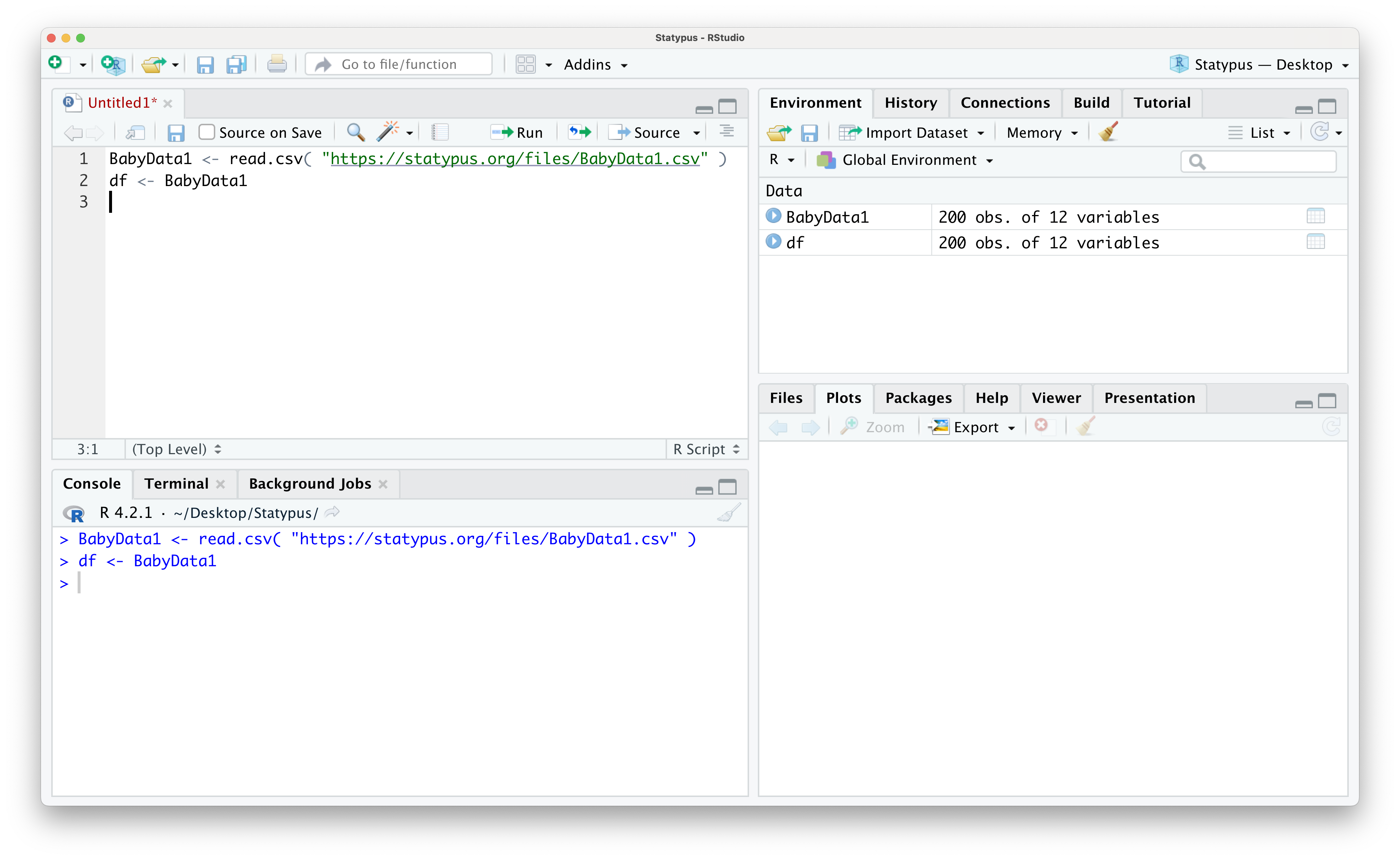
Figure 1.49: Making a Working Copy
Here we see that both BabyData1 and df are data frames made up of 200 observations (individuals) of 12 variables and further investigation would show the files are identical. We give an example by showing the contents of df$sex below.
##   [1] "F" "F" "F" "F" "F" "M" "F" "M" "M" "M" "F" "F" "M" "F" "M" "M" "F" "F"
##  [19] "F" "F" "M" "F" "F" "F" "M" "M" "M" "M" "F" "F" "M" "M" "M" "F" "F" "M"
##  [37] "F" "M" "M" "M" "M" "M" "M" "M" "M" "F" "M" "F" "M" "F" "F" "F" "M" "F"
##  [55] "M" "M" "M" "F" "M" "F" "F" "F" "M" "M" "M" "M" "F" "F" "M" "M" "M" "F"
##  [73] "M" "F" "M" "F" "F" "M" "F" "F" "M" "M" "F" "F" "M" "F" "M" "F" "F" "F"
##  [91] "F" "M" "M" "F" "F" "F" "F" "F" "M" "M" "M" "M" "M" "M" "F" "M" "M" "F"
## [109] "M" "M" "M" "M" "M" "M" "F" "M" "F" "F" "M" "F" "M" "F" "F" "F" "M" "F"
## [127] "M" "F" "M" "M" "F" "F" "F" "M" "M" "M" "M" "F" "F" "F" "M" "F" "F" "M"
## [145] "F" "F" "F" "F" "F" "F" "F" "M" "M" "M" "F" "M" "F" "M" "M" "F" "F" "F"
## [163] "M" "M" "F" "F" "M" "M" "F" "F" "M" "M" "M" "M" "F" "F" "F" "M" "M" "M"
## [181] "F" "M" "F" "M" "M" "M" "M" "M" "F" "F" "F" "M" "F" "M" "F" "F" "M" "M"
## [199] "M" "M"
From here, it is recommended that you do all of your work with the df copy and leave BabyData1 alone. For example, we could now replicate the following line of code
with the more concise line shown below.
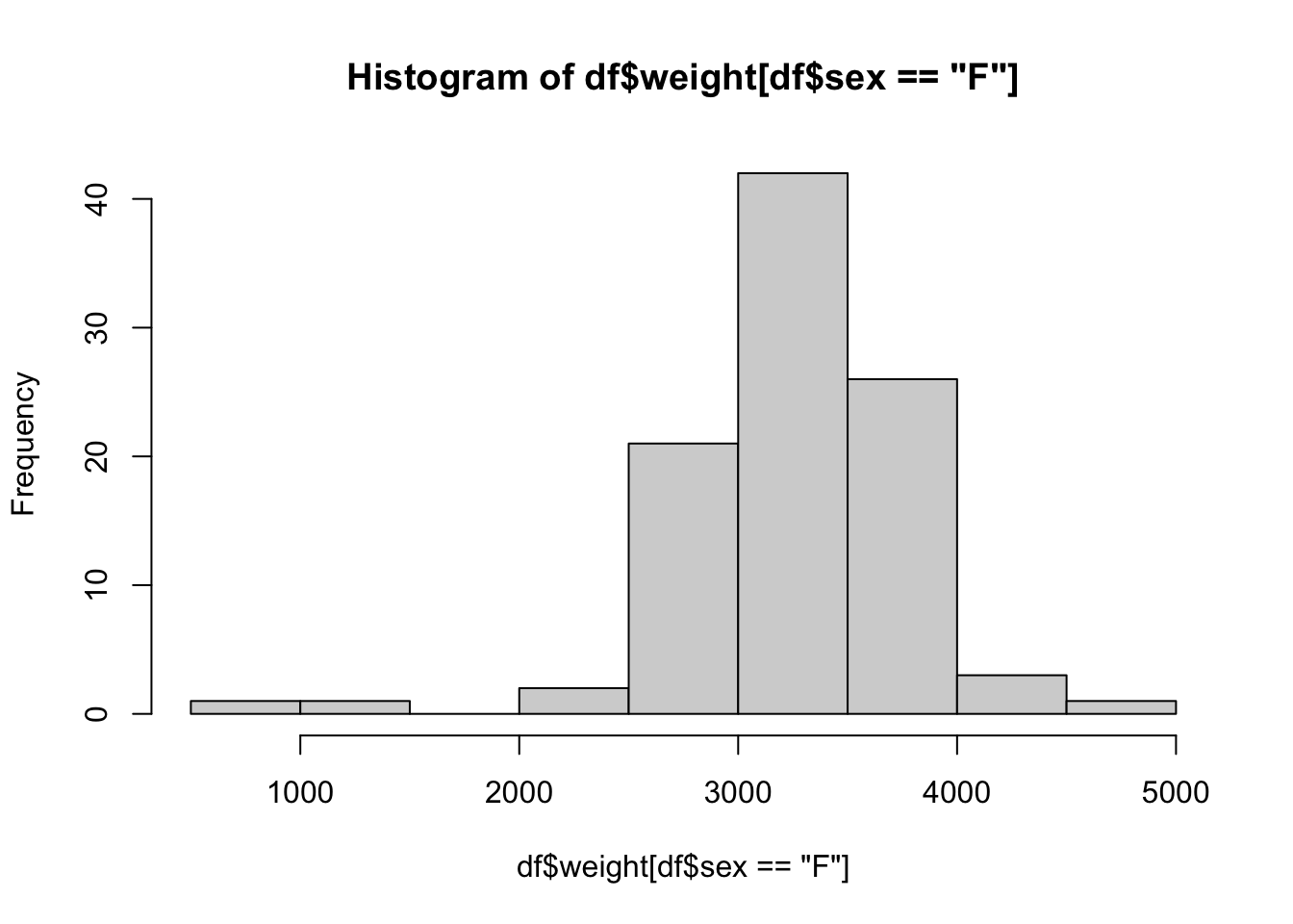
Moreover, if you were to make the mistake of using the equal sign assignment operator like we did in Example 1.30, we can now easily fix it. We show this now by first intentionally “corrupting” df$sex and then looking at it
##   [1] "F" "F" "F" "F" "F" "F" "F" "F" "F" "F" "F" "F" "F" "F" "F" "F" "F" "F"
##  [19] "F" "F" "F" "F" "F" "F" "F" "F" "F" "F" "F" "F" "F" "F" "F" "F" "F" "F"
##  [37] "F" "F" "F" "F" "F" "F" "F" "F" "F" "F" "F" "F" "F" "F" "F" "F" "F" "F"
##  [55] "F" "F" "F" "F" "F" "F" "F" "F" "F" "F" "F" "F" "F" "F" "F" "F" "F" "F"
##  [73] "F" "F" "F" "F" "F" "F" "F" "F" "F" "F" "F" "F" "F" "F" "F" "F" "F" "F"
##  [91] "F" "F" "F" "F" "F" "F" "F" "F" "F" "F" "F" "F" "F" "F" "F" "F" "F" "F"
## [109] "F" "F" "F" "F" "F" "F" "F" "F" "F" "F" "F" "F" "F" "F" "F" "F" "F" "F"
## [127] "F" "F" "F" "F" "F" "F" "F" "F" "F" "F" "F" "F" "F" "F" "F" "F" "F" "F"
## [145] "F" "F" "F" "F" "F" "F" "F" "F" "F" "F" "F" "F" "F" "F" "F" "F" "F" "F"
## [163] "F" "F" "F" "F" "F" "F" "F" "F" "F" "F" "F" "F" "F" "F" "F" "F" "F" "F"
## [181] "F" "F" "F" "F" "F" "F" "F" "F" "F" "F" "F" "F" "F" "F" "F" "F" "F" "F"
## [199] "F" "F"
Now, instead of having to remove df, we can just recreate it with df <- BabyData1 since we haven’t modified BabyData1 at all.
In fact, all you need to do is place your cursor on the line with df <- BabyData1 and rerun that line. We verify this “fix” worked by once again looking at the contents of df$sex.
##   [1] "F" "F" "F" "F" "F" "M" "F" "M" "M" "M" "F" "F" "M" "F" "M" "M" "F" "F"
##  [19] "F" "F" "M" "F" "F" "F" "M" "M" "M" "M" "F" "F" "M" "M" "M" "F" "F" "M"
##  [37] "F" "M" "M" "M" "M" "M" "M" "M" "M" "F" "M" "F" "M" "F" "F" "F" "M" "F"
##  [55] "M" "M" "M" "F" "M" "F" "F" "F" "M" "M" "M" "M" "F" "F" "M" "M" "M" "F"
##  [73] "M" "F" "M" "F" "F" "M" "F" "F" "M" "M" "F" "F" "M" "F" "M" "F" "F" "F"
##  [91] "F" "M" "M" "F" "F" "F" "F" "F" "M" "M" "M" "M" "M" "M" "F" "M" "M" "F"
## [109] "M" "M" "M" "M" "M" "M" "F" "M" "F" "F" "M" "F" "M" "F" "F" "F" "M" "F"
## [127] "M" "F" "M" "M" "F" "F" "F" "M" "M" "M" "M" "F" "F" "F" "M" "F" "F" "M"
## [145] "F" "F" "F" "F" "F" "F" "F" "M" "M" "M" "F" "M" "F" "M" "M" "F" "F" "F"
## [163] "M" "M" "F" "F" "M" "M" "F" "F" "M" "M" "M" "M" "F" "F" "F" "M" "M" "M"
## [181] "F" "M" "F" "M" "M" "M" "M" "M" "F" "F" "F" "M" "F" "M" "F" "F" "M" "M"
## [199] "M" "M"
This is another great reason to use R scripts!
Review for Chapter 1
Chapter 1 Quiz: Introduction to R
This quiz tests your understanding of the RStudio environment, basic R syntax, and core data structures presented in Chapter 1. The answers can be found prior to the Exercises section.
True or False: RStudio is the Integrated Development Environment (IDE) that is designed to make the command-line statistical software R easier to use.
True or False: The Console pane, located in the bottom-left section of RStudio, is where you enter and execute single lines of code directly.
True or False: In R, the
rm()function is primarily used to combine multiple arguments into a single vector.True or False: The History pane, found in one of the right sections of RStudio, displays all of the data objects, vectors, and data frames currently stored in memory.
True or False: A key difference between an Error and a Warning is that a Warning prevents R from completing the requested task, while an Error allows the task to be completed but notes a potential issue.
True or False: In R, the three basic data types are Numeric, Character (Strings), and Logical.
True or False: The dollar sign operator.
$, is the most straightforward way to access a specific column (variable) within a data frame in R.True or False: An R Package only needs to be installed once on a computer, and the
library()command never needs to be run again, even after restarting RStudio.True or False: A vector is a data structure in R that can only store one type of basic data (e.g., only Numeric or only Character).
True or False: Typing a question mark followed by a function name (e.g.,
?hist) into the Console will open the built-in help file for that function.
Definitions
Section 1.2
Section 1.3
Definition 1.2 \(\;\) A Vector is an ordered collection of values of a similar type of data. Each value in a vector is known as an Entry and the position of each entry is known as the entry’s Index or Indices if dealing with more than one index. The total number of entries is known as the Length of the vector. The first entry has an index of 1, the second entry has an index of 2, and finishes with the last entry having an index matching the length of the vector.
Definition 1.3 \(\;\) The Left Arrow Assignment Operator or simply the Left Arrow Operator, <-, is used to assign a value to a name. It can be created by combining the less than character < with a dash -. We recommend that you place a space before and after the left arrow operator.
Definition 1.4 \(\;\) The bracket operator can be applied to vectors and other data formats to extract or replace parts.
Definition 1.5 \(\;\) A CSV File is a computer text file that ends in the .csv extension. The term CSV stands for Comma-Separated Values.
A CSV file is robust enough to work in industrial statistical software such as R or even the more familiar spreadsheet applications like Microsoft Excel.
Definition 1.6 \(\;\) A Data Frame is a list of variables of the same number of rows. A data frame is thus a collection of different variables each of which is contained in its own column.
Definition 1.7 \(\;\) While there are more nuanced ways of accessing information within a data frame, the dollar sign operator, $, is the easiest way to access values in a data frame.
If we have a data frame named df, then typing df$ into a script or into the Console should bring up a drop down menu of the variables contained in the data frame.
Big Ideas
Section 1.3
Most people begin their interaction with variables using the letter \(x\) for everything. The phrase “Solve for \(x\)” can even cause trepidation in some hearts. We are certainly able to use \(x\) here, but we note that it will appear as x in R.
However, R allows us the flexibility to name variables nearly anything we want. For example, in Example 1.3 we used the variable name phi for the Greek letter \(\varphi\). In Chapter 4 we will introduce the sample mean which we will denote \(\bar{x}\) which is read as “\(x\)-bar” and we will store values in RStudio as xbar.
In general, you should use variable names that are descriptive and representative of what they are labeling. There are a few rules, however. Variable names cannot begin with a number or a “dot”27, .. You can combine words with juxtaposition such as MeanOfSample or MassOfSpring or with the underscore character, _, such as Mean_Of_Sample or Mass_Of_Spring.
We will introduce Data Frames in Section 1.3.4 and at times will save a copy of a data frame we are working with as df or dd to simplify or shorten some code. We call this a Working Copy of a data frame and discuss it in Section 1.5.6
In Example 1.12, use used the bracket operator with an enclosed inequality to extract just those entries that satisfied the inequality snickers < 50. To see how this works, we look at what happens if we just run the inequality in RStudio.
##   [1] FALSE FALSE FALSE FALSE FALSE FALSE FALSE FALSE FALSE FALSE FALSE FALSE
##  [13] FALSE FALSE  TRUE FALSE FALSE FALSE FALSE FALSE FALSE FALSE FALSE FALSE
##  [25] FALSE FALSE FALSE FALSE FALSE FALSE FALSE FALSE FALSE FALSE FALSE FALSE
##  [37] FALSE FALSE FALSE FALSE FALSE FALSE FALSE FALSE FALSE FALSE FALSE FALSE
##  [49] FALSE FALSE FALSE FALSE FALSE FALSE  TRUE FALSE FALSE FALSE FALSE FALSE
##  [61] FALSE FALSE FALSE FALSE  TRUE FALSE  TRUE FALSE FALSE FALSE FALSE FALSE
##  [73] FALSE FALSE FALSE FALSE FALSE  TRUE FALSE FALSE FALSE FALSE FALSE FALSE
##  [85] FALSE FALSE FALSE FALSE FALSE FALSE FALSE  TRUE FALSE FALSE FALSE FALSE
##  [97] FALSE  TRUE FALSE FALSE
We see that the result is a vector of logical values where the \(k^\text{th}\) entry is the logical result of testing if the \(k^\text{th}\) entry of snickers is strictly less than 51. For example, snickers[ 1 ] was 51.1 which is not less than 51 so the first entry of this new vector is FALSE. Moreover, snickers[ 15 ]was 50.8 which is less than 51 so the fifteenth entry of the above logical vector is TRUE. When we put this logical vector into the brackets after snickers, it will keep the entries with indices that are TRUE and omit the values that are FALSE.
You can use the following logical “test operators” to do similar tests:
>: Tests if the left hand side is strictly greater than the right hand side.<=: Tests if the left hand side is less than or equal to the right hand side.>=: Tests if the left hand side is greater than or equal to the right hand side.==: Tests if the left hand side is equal to the right hand side.!=: Tests if the left hand side is not equal to the right hand side.
If the data is hosted on a web page, it is much easier to do a “direct download” of it using the read.csv() function. We will not go into the nuances of read.csv() here, but we will utilize it to expedite the loading of data onto our machine..
Direct downloads like above will be the primary method used to open new datasets on Statypus. We will do so via purple “Data Download” boxes like the one we used for snickers, but a more typical usage of it is in Example 1.15
The dollar sign operator is a very useful tool for accessing values in a data frame, but there are more robust tools we can use. We can use the bracket operator, [ ], that we first used for vectors in Example 1.12 again for data frames to pull out subsets of the data frame. When we used the bracket operator for vectors, we only had to provide one input within the brackets. Now that we are using it for a data frame, we must pass it two different inputs. For discussion purposes, we will call these inputs R and C and they should be entered as df[ R, C] where df is the name of the data frame we are utilizing. The R input is what we will call the Row Rules and the C input is what we will call the Column Rules. Example 1.18 shows some examples of using these rules.
Section 1.4
In Example 1.9 we ran the following line of code: sort( snickers, decreasing = TRUE ). This is an example of running an R function and shows the basic syntax we will use, which is shown below.
functionName( argument1, argument2, argument3 )In R, functions can have more than one input (called arguments), we show 3 above, but it can be more. Moreover, those arguments can at times be long to type out so that the above syntax may stretch well across your computer screen. If we wanted to make the code a little easier to read, we could rewrite the above syntax as follows:
functionName( argument1,
argument2,
argument3 )When looking at the above, when R gets to the first parenthesis, (, it knows to begin looking for arguments for functionName and it continues to do so until it hits the closing parenthesis, ). Regardless of how you type it out on the screen, you should have a comma after each argument except for the last one which should be followed by ).
We can see what arguments a function wants by typing in the function, such as sort(), into an R script (or in the Console) and waiting. A yellow pop-up will appear showing the arguments that the function needs passed to it.
Figure 1.50: The pop-up showing the arguments of sort()
This shows that the main arguments are x, the data to be sorted, and decreasing which is set to FALSE by default as indicated in the pop-up. The ellipsis indicates that there are other, and lesser used, arguments which we can look at by using the help option by running ?sort.
Section 1.5
A lot of mistakes can be avoided if the user starts a new “session” of RStudio each time they interact with this. To do this, make sure to do the following steps each time you are done working in RStudio.
1. Save any open R script.
For example, the following screenshot shows us working with the “GoldenRatio.R” R script we built in Example 1.3 and if you look in the tabs of the upper left pane, you will see that “GoldenRatio.R” is displayed in red indicating that it needs saved. You should save it by using the “Save current document” icon (which resembles a computer diskette) which appears directly below the .R of “GoldenRatio.R” below.
Figure 1.51: The help file of sort()
2. Shut down RStudio
Once you have saved all of your open documents, it is time to shut down RStudio. When you do so, you should see a dialog box like the following appear.
Figure 1.52: The help file of sort()
At this point, we come to the most important step.
3. Make certain to select Don't Save on the dialog box shown above.
At Statypus, we highly encourage the Type Three Rule. That is, you should type the first three characters of the element you are looking for and then using the menu to select the appropriate value.
If you begin typing (at least the first three characters of) something into RStudio, auto-complete will search for all things in memory, data or functions, in a non-case-sensitive way and allow you to choose from a drop down list. For example, typing vie into an R script or into the R console it will pop up a menu to allow you to choose the function, View(), as shown below.
Figure 1.53: Autocomplete Example
If there are more than one option for the three characters for what you type, you get a dropdown menu showing all of the objects that begin with that regardless of case. For example, below is what you will likely see if you type in bar into R.
Figure 1.54: Autocomplete Example
From here, you can choose the function you, maybe the function barplot() which we will introduce in Chapter 3.
Users new to working with computer software that requires them to enter code into a terminal manually like we do with R may be a bit confused about the distinction between parentheses, ( ), and brackets, [ ]. In most students’ experience, these grouping symbols have been used interchangeably in their previous math coursework. However, R is very particular about every symbol that the user offers it. It is possible that students would be quite comfortable with the expression \(f(x)\), but may be perplexed if they saw it written as \(f[x]\). This will be our mental trick to remembering when to use parentheses. We will always use parentheses following a function.
We have seen that the two sets of grouping symbols, ( ) and [ ], serve very different purposes and must be kept straight by the user.
Parentheses
The parentheses can be used as as typical grouping symbols when making calculations such as when we calculated the Golden Ratio in Example 1.5 with the following line of code.
As we saw in Section @(), we also use parentheses to hold the arguments we want to pass to a function like the “mock” code shown below.
functionName( argument1 )Brackets
The bracket operator, however, should not follow a function, but a piece of data such as a vector or data frame.
For vectors, we use a single logical rule as shown in the “mock” code below.
vector[ Rule ]For data frames, we use two different logical rules as shown below in “mock” code.
df[ R, C ]Here R is rule applied to the rows and C is the rule applied to columns. As we will see in Example 3.6, a rule can be made up of more than one logical test if we combine them with the Logical And Operator, &, or the Logical Or Operator, |.
As we saw in Example 1.29, missing values can cause surprising results from functions. The correct way to handle missing values varies by the function which we will discuss in the coming chapters.
In general, however, a result of NA is simply R’s way of telling us that some data value is missing and it is up to us as the user to decide if we want to take further measures to get a different result.
Example 1.30 motivates this Big Idea. If you are doing any major manipulation work with a dataset, it may be advisable to create a Working Copy of the it. For example, consider the block of code below.
The first line of code loads BabyData1 into our Environment from the URL shown. The second line of code then creates a new data frame named df by making a copy of BabyData1. This is shown in the following screenshot.
Figure 1.55: Making a Working Copy
Here we see that both BabyData1 and df are data frames made up of 200 observations (individuals) of 12 variables and further investigation would show the files are identical. We give an example by showing the contents of df$sex below.
##   [1] "F" "F" "F" "F" "F" "M" "F" "M" "M" "M" "F" "F" "M" "F" "M" "M" "F" "F"
##  [19] "F" "F" "M" "F" "F" "F" "M" "M" "M" "M" "F" "F" "M" "M" "M" "F" "F" "M"
##  [37] "F" "M" "M" "M" "M" "M" "M" "M" "M" "F" "M" "F" "M" "F" "F" "F" "M" "F"
##  [55] "M" "M" "M" "F" "M" "F" "F" "F" "M" "M" "M" "M" "F" "F" "M" "M" "M" "F"
##  [73] "M" "F" "M" "F" "F" "M" "F" "F" "M" "M" "F" "F" "M" "F" "M" "F" "F" "F"
##  [91] "F" "M" "M" "F" "F" "F" "F" "F" "M" "M" "M" "M" "M" "M" "F" "M" "M" "F"
## [109] "M" "M" "M" "M" "M" "M" "F" "M" "F" "F" "M" "F" "M" "F" "F" "F" "M" "F"
## [127] "M" "F" "M" "M" "F" "F" "F" "M" "M" "M" "M" "F" "F" "F" "M" "F" "F" "M"
## [145] "F" "F" "F" "F" "F" "F" "F" "M" "M" "M" "F" "M" "F" "M" "M" "F" "F" "F"
## [163] "M" "M" "F" "F" "M" "M" "F" "F" "M" "M" "M" "M" "F" "F" "F" "M" "M" "M"
## [181] "F" "M" "F" "M" "M" "M" "M" "M" "F" "F" "F" "M" "F" "M" "F" "F" "M" "M"
## [199] "M" "M"
From here, it is recommended that you do all of your work with the df copy and leave BabyData1 alone. For example, we could now replicate the following line of code
with the more concise line shown below.

Moreover, if you were to make the mistake of using the equal sign assignment operator like we did in Example 1.30, we can now easily fix it. We show this now by first intentionally “corrupting” df$sex and then looking at it
##   [1] "F" "F" "F" "F" "F" "F" "F" "F" "F" "F" "F" "F" "F" "F" "F" "F" "F" "F"
##  [19] "F" "F" "F" "F" "F" "F" "F" "F" "F" "F" "F" "F" "F" "F" "F" "F" "F" "F"
##  [37] "F" "F" "F" "F" "F" "F" "F" "F" "F" "F" "F" "F" "F" "F" "F" "F" "F" "F"
##  [55] "F" "F" "F" "F" "F" "F" "F" "F" "F" "F" "F" "F" "F" "F" "F" "F" "F" "F"
##  [73] "F" "F" "F" "F" "F" "F" "F" "F" "F" "F" "F" "F" "F" "F" "F" "F" "F" "F"
##  [91] "F" "F" "F" "F" "F" "F" "F" "F" "F" "F" "F" "F" "F" "F" "F" "F" "F" "F"
## [109] "F" "F" "F" "F" "F" "F" "F" "F" "F" "F" "F" "F" "F" "F" "F" "F" "F" "F"
## [127] "F" "F" "F" "F" "F" "F" "F" "F" "F" "F" "F" "F" "F" "F" "F" "F" "F" "F"
## [145] "F" "F" "F" "F" "F" "F" "F" "F" "F" "F" "F" "F" "F" "F" "F" "F" "F" "F"
## [163] "F" "F" "F" "F" "F" "F" "F" "F" "F" "F" "F" "F" "F" "F" "F" "F" "F" "F"
## [181] "F" "F" "F" "F" "F" "F" "F" "F" "F" "F" "F" "F" "F" "F" "F" "F" "F" "F"
## [199] "F" "F"
Now, instead of having to remove df, we can just recreate it with df <- BabyData1 since we haven’t modified BabyData1 at all.
In fact, all you need to do is put your cursor on the line containing df <- BabyData1 and rerun that line. We verify this “fix” worked by once again looking at the contents of df$sex.
##   [1] "F" "F" "F" "F" "F" "M" "F" "M" "M" "M" "F" "F" "M" "F" "M" "M" "F" "F"
##  [19] "F" "F" "M" "F" "F" "F" "M" "M" "M" "M" "F" "F" "M" "M" "M" "F" "F" "M"
##  [37] "F" "M" "M" "M" "M" "M" "M" "M" "M" "F" "M" "F" "M" "F" "F" "F" "M" "F"
##  [55] "M" "M" "M" "F" "M" "F" "F" "F" "M" "M" "M" "M" "F" "F" "M" "M" "M" "F"
##  [73] "M" "F" "M" "F" "F" "M" "F" "F" "M" "M" "F" "F" "M" "F" "M" "F" "F" "F"
##  [91] "F" "M" "M" "F" "F" "F" "F" "F" "M" "M" "M" "M" "M" "M" "F" "M" "M" "F"
## [109] "M" "M" "M" "M" "M" "M" "F" "M" "F" "F" "M" "F" "M" "F" "F" "F" "M" "F"
## [127] "M" "F" "M" "M" "F" "F" "F" "M" "M" "M" "M" "F" "F" "F" "M" "F" "F" "M"
## [145] "F" "F" "F" "F" "F" "F" "F" "M" "M" "M" "F" "M" "F" "M" "M" "F" "F" "F"
## [163] "M" "M" "F" "F" "M" "M" "F" "F" "M" "M" "M" "M" "F" "F" "F" "M" "M" "M"
## [181] "F" "M" "F" "M" "M" "M" "M" "M" "F" "F" "F" "M" "F" "M" "F" "F" "M" "M"
## [199] "M" "M"
This is another great reason to use R scripts!
Important Alerts
Section 1.1
While there are many good reasons to utilize the online posit.cloud option of RStudio, we will default to discussions on Statypus where we assume that the user is working with a downloaded copy. If you are struggling to utilize something on Statypus due to this issue, please check the help files at posit.cloud or email the author at phil.huling@slu.edu.
Section 1.2
New users may mistakenly try to use R through the R software directly. Doing so is definitely possible, but the use of RStudio is highly recommended. If you see a window like the one below, close that application and make sure you search your computer for “RStudio” and try again.
Figure 1.56: R GUI
Section 1.3
Choose your variable names with care, however, as variable names are case sensitive. We discuss this in a Big Idea at the beginning of Section 1.5.2.
You should not use variable names that could conflict with existing R objects. These can be single letters as below.
Do not use: c, q, t, C, D, I, T, F
These letters have built in uses within R and assigning variables to them can cause issues. Further, certain names should be avoided as they may align with functions such as the ones below.
Do not use: sample, sum, mean
We will actually deal with two types of numerical data. For example, in Example 1.11, we saw that the snickers dataset was a vector of length 100 containing numeric values as indicated by the num in either the output of str( snickers ) or as seen in the environment as shown in Figure 1.27. If the numeric data we are dealing with only contains integers, it may actually be of the int or integer type. Fortunately, the user does not need to worry about the distinction and R will do calculations with both types simultaneously without the user ever knowing.
Most arithmetic and algebra books allow juxtaposition to be used for a short hand for multiplication. For example, in most math classes we take the symbols \(13y\) to mean 13 times the variable \(y\). However, this does not work in R. Moreover, attempts to use a space between the values, 13 y, or to use parentheses, 13(y), will also fail to give the desired product.
You must use the star operator to multiply objects in R.
Important Remarks
Section 1.2
The output we saw for the calculation given by (1 + sqrt(5))/2 in Example 1.3 above produced the output of [1] 1.618034 in the Console.
However, if we were to display that in this book without the use of screen shots, it would look something like this:
## [1] 1.618034The characters ## indicate that what follows is the output of R code. These characters are not part of the output, but simply a way that R communicates what is output when producing a document like this. You will see the ## characters preceding nearly every output in Statypus.
Section 1.3
It is very important to note that when we saved the blood type in Example 1.8 that we contained the character string in quotation marks. Failure to do so will cause an error and we will see the result of this in Example 1.21 in Section 1.5.3.
Unless you have redefined the values of T or F, these values are shortcuts to the values of TRUE and FALSE respectively.
There is a bit of a debate about whether to use the left arrow operator, <-, or a single equal sign, =. While the two are nearly interchangeable, there are places where = cannot be used and on Statypus we will only use = for defining arguments within functions or when we define variables before a block of code where we want to mirror the idea of a function.
In addition, using the left arrow operator makes a clear distinction on where the value and name should be in relation to the operator. While x = 2 is equivalent to x <- 2, look what happens if we reverse the order.
## Error in `2 = x`:
## ! invalid (do_set) left-hand side to assignment
R was unable to complete our request and gave us an Error, a topic we will more fully investigate in Section 1.5.3.
Note that Definition 1.2 explicitly requires all entries have the same data type. If you attempt to combine mixed varieties of data with c(), R will do its best to create a vector of a single type. Turning numeric values into character strings is one of the most likely outcomes of trying to mix data types. For example, consider the code below trying to combine 1 and the letter "B".
## [1] "1" "B"To avoid the conflicting types of data, R automatically turned the numeric value of 1 into the character string "1" as we see in the output.
If we saved this vector as vec with the following code
would show the following in the environment making it clear that vec is a vector of character strings.
Figure 1.57: Looking at Data in the Environment
Section 1.4
Functions can also have more than one output. This may go against the definition of a function that you learned, but the most important concept is still true. The output of a function is uniquely determined by the arguments that we pass to the function.28
Section 1.5
One of the benefits of loading data and functions from packages is that they are required to have help files which can be accessed with the question mark operator. For example, if you installed the HistData package like we discussed in Section 1.3.5, you could find more info about the DrinkWages data frame by running ?DrinkWages in either a script or the Console.
Many typos can be avoided by following the Rule of Type Three as R is case-sensitive so that view( snickers ) causes an error while View( snickers ) will display the vector snickers in the upper left pane of RStudio (assuming it has been loaded like we did in Example 1.9).
## Error in `view()`:
## ! could not find function "view"
New Functions
Section 1.2
Section 1.3
The syntax of c() is
where the arguments are objects to be concatenated. All NULL entries are dropped unless at the very beginning of the argument list.
The syntax of head() is
where the argument is:
x: An R object.
Quiz Answers
True
True
False (The
c()function combines arguments;rm()removes objects.)False (The Environment pane displays stored objects.)
False (The definitions are reversed: Errors prevent completion; Warnings allow completion.)
True
True
False (The
library()command must be used to reload the package every time R is started.)True
True
Exercises
Exercise 1.1 For each of the following parts, identify where the student went wrong and find a way to fix their code. Feel free to run the code as it is to see what Errors or Warnings appear.
- A student wants to save the value of the square root of \(\pi\) to his computer as an object named
SPiusing the following line of code.
- While trying to save the value of the Golden Ratio with the code below, a student was left with R giving them a
+prompt in their console.
- A student was trying to access the fuel efficiencies of only 4 cylinder cars with the following line of code.
- A student was trying to define a vector of the names of the primary colors with the following line of code.
Exercise 1.2 Use R’s basic arithmetic operations to answer the following:
- Calculate the result of \(150\) divided by \(12\).
- Assign the result of \(\left(4^3 + 15\right) / 2\) to an object named
Bob. - Assign the result of \(\sqrt{144}\) to an object named
SqRoot. (Hint: You can use thesqrt()function or raise to the power of \(0.5\)). - Using the results of parts b. and c., calculate the value of
Bob - SqRoot.
Exercise 1.3 Practice combining and accessing elements within vectors:
- Create a vector named
Weightscontaining the following values: \(155, 140, 182, 160, 195\). - Use the bracket operator to access and display only the third element of the
Weightsvector. - Use the
sum()function to calculate the total weight of all elements in theWeightsvector. - Use the appropriate function to calculate the average (mean) weight.
Exercise 1.4 Answer the following questions regarding R code execution and library management:
- If you try to execute the code
MyVariable <- 5 +, R will return an “unexpected end of input” message. Is this an Error or a Warning, and why? - If you assign the character value
"Statypus"to an object namedCourseName, what would thestr(CourseName)function report as the data type? - When you run
length(c(1, 2, 3, 4))in the console, what value does R return?
Exercise 1.5 Answer the following questions about the RStudio environment and basic command usage:
Identify the four main panes in the default RStudio layout (Source, Console, Environment/History, and Files/Plots/Packages/Help) and briefly describe the primary purpose of each (e.g., The Console is where R commands are executed).
Which RStudio pane displays the objects (data, variables, functions) currently stored in the computer’s memory?
In the R Markdown chunk below, identify what each line of code does.
Explain the difference between an Error and a Warning message in R, based on the chapter’s definitions.
Exercise 1.6 Practice using the assignment operator (<-) and basic arithmetic:
- Assign the value of \(7 + 12\) to a new object named
Alpha. - Assign the value of \(5\) squared, \(5^2\), to a new object named
Beta. - Create a third object,
Gamma, that is equal to the sum ofAlphaandBeta. - Execute the single R command needed to remove the object
Betafrom the RStudio environment.
Exercise 1.7 Use the functions introduced in the chapter to inspect and combine data:
- Use the
c()function to create a single vector namedAgescontaining the following numbers: \(18, 20, 19, 21, 18, 22\). - Use the
head()function to view the first few values of theAgesvector you just created. Explain why usinghead()on a small vector like this might not be very informative. - Use the
length()function on theAgesvector to confirm the number of elements it contains. - Use the
str()function on theAgesvector. What is the data type (e.g., numeric, integer, character) that R reports for this vector?
1.6 Appendix
1.6.1 Setting Up Your AI Lab Partners
To assist with your work in this course, we will utilize AI tools integrated directly into RStudio. Think of GitHub Copilot as your “autofill” for code.
GitHub Copilot is an AI programmer that suggests code as you type. It is particularly helpful for learning base R syntax because it predicts the functions you need based on your comments. You should check if your school has a free Copilot subscription for students. If not, you can sign up for a free account with GitHub Education.
- Sign Up: Go to GitHub Education and verify your student status to get Copilot for free.
- Enable in RStudio: * Open RStudio and navigate to
Tools>Global Options>Copilot.- Check the box labeled “Enable GitHub Copilot”.
- Click “Sign In” and follow the prompts to link your GitHub account.
- Usage: When you see “Ghost Text” (light gray code) appearing in your script, simply press the Tab key to accept the suggestion.
While these AI tools are incredibly powerful, they are not perfect. Always verify the code they suggest. In this course, we prioritize Base R. If an AI suggests a package you haven’t seen yet (like dplyr), you can tell it: “Please provide the solution using only Base R functions.”
Shaw, George; Nodder, Frederick Polydore (1799). “The Duck-Billed Platypus, Platypus anatinus”. The Naturalist’s Miscellany. 10 (CXVIII): 385–386↩︎
While not universally agreed upon, we have chosen to always italicize R when it refers to the statistical package.↩︎
R Core Team (2022). R: A language and environment for statistical computing. R Foundation for Statistical Computing, Vienna, Austria. URL https://www.R-project.org/.↩︎
The first commercial Beta version of RStudio was made available on February 28, 2011 and it wasn’t until January of 2016 that version 1.0 would be made commercially available.↩︎
Don’t let the terms integrated development environment or programming language scare you too much at this point. The entire aim of Statypus is to make the use of computers within statistics as easily learned as possible.↩︎
We won’t get too pedantic just yet, but the curious reader can see Wikipedia if they are curious about what we mean by the principal square root.↩︎
In a loose sense, the Golden Ratio gives the ratio of the sides of a rectangle that is the “most rectangular.” In other words, if the ratio was closer to 1, the rectangle would look more squarish and if the ratio was larger, the rectangle would look longer like a strip.↩︎
There is no “Fo” or “Fum” here. Sorry to all those fans of Jack or possibly even Apollo 17.↩︎
For those of you who found this footnote, don’t mind the Droste Effect of Figure 1.10.↩︎
We won’t get into the debate of the name of this character here. Feel free to make that call yourself.↩︎
Such as Edward J. Goodwin did in his attempt to pass the infamous “Indiana Pi Bill.”↩︎
Yes, this is the correct spelling of the number. The popular website www.Google.com derives its name from the number, but this was due to a misspelling.↩︎
The use of “dot-names” or variables beginning with a
.are “hidden” or “invisible” by default. The help file ofls()can be accessed using?lsmentions this under theall.namesargument. This can be utilized by advanced users for many purposes, but it is not recommended unless you have a specific reason why you want the files to be hidden.↩︎Unless you have Triskaidekaphobia, in which case, use 17 instead!↩︎
This is really kilocalories or “large calories.” See Wikipedia for more information.↩︎
We will dive into this much more later, but the curious reader can see the note following Example 4.18 in Section 4.4.1 or the footnote in Example 5.8 in Section 5.4.↩︎
One may argue that some of the “random” functions we will use, such as
sample()andrnorm(), violate this concept. However, this is not the case as these functions also call on a “hidden” argument which is the “seed” it uses to create what we infer as a random value. The user can use theset.seed()function to choose the seed value prior to running a random function and the results will be consistent. This is especially useful when doing something such as writing a textbook when you want to be able to discuss the results of a function and not have it change when you recompile the book.↩︎In a bit of irony, we recommend using
?helpto look at how to use more advanced functionality ofhelp()if you are so inclined.↩︎Wikipedia gives a good quick discussion to the origins of this terminology.↩︎
YouTube has a great video where Tom Scott discusses the “onosecond” caused by the worst typo he ever made.↩︎
In a bit of irony, we recommend using
?helpto look at how to use more advanced functionality ofhelp()if you are so inclined.↩︎The use of “dot-names” or variables beginning with a
.are “hidden” or “invisible” by default. The help file ofls()can be accessed using?lsmentions this under theall.namesargument. This can be utilized by advanced users for many purposes, but it is not recommended unless you have a specific reason why you want the files to be hidden.↩︎One may argue that some of the “random” functions we will use, such as
sample()andrnorm(), violate this concept. However, this is not the case as these functions also call on a “hidden” argument which is the “seed” it uses to create what we infer as a random value. The user can use theset.seed()function to choose the seed value prior to running a random function and the results will be consistent. This is especially useful when doing something such as writing a textbook when you want to be able to discuss the results of a function and not have it change when you recompile the book.↩︎