Chapter 6 From Proportions to Probabilities
Figure 6.1: A Statypus Playing Dice
The platypus only naturally exists along the coast of Eastern Australia. In fact, the only place that a platypus can be found outside of Australia is at the San Diego Zoo Safari Park. They are best friends with the giant pandas that live there as well! (The last statement is false, but I wish it was true.)60
The goal of probability and statistics is to understand the real world. Many of the situations we face on a daily basis involve a certain amount of chance. The time it takes to drive to the store can greatly be affected by the amount of traffic on the roads or simply the timing of the traffic signals along your path. Modern cell phones are incredibly resilient, but every drop offers the chance that it may break or become damaged. Even our births have an element of chance as certain proportions of people are born with life threatening conditions, such as trisomy 13, based on random genetic “mistakes” made while duplicating the genetic code.
Probability experiments in the real world are usually slow and often expensive. Instead of running real world experiments, it is easier to model these experiments and then use a computer to imitate the results. This process goes by several names, such as stochastic simulation, Monte Carlo simulation or probability simulation. Since this is the only type of simulation we will discuss, we simply call it simulation.
New R Functions Used
All functions listed below have a help file built into RStudio. Most of these functions have options which are not fully covered or not mentioned in this chapter. To access more information about other functionality and uses for these functions, use the ? command. E.g. To see the help file for sample(), you can run ?sample or ?sample() in either an R Script or in your Console.
We will see the following functions in Chapter 6.
sample(): Takes a sample of the specifiedsizefrom the elements ofxusing either with or without replacement.
We first saw sample() in Chapter 2, but revisit it here and look at it more robustly.
To load all of the datasets used in Chapter 6, run the following line of code.
Remember that R uses case sensitive file names. As such, there are two different vectors in this chapter relating to the Snickers candy bar. Both vectors contian data about the same 100 Snickers bars where snickers contains the mass of each bar in grams and Snickers contains the calculated weight of each bar in ounces using a conversion rate of 28.35 grams to each ounce.
6.1 Proportion or Probability?
Games of chance are a staple of childhood and allow players of different ages to compete fairly. Games such as “Candy Land” require no skill as there is no strategy that can be employed to gain an advantage. Games such as “Snakes and Ladders” are even more complex, but again the outcome of the game is completely determined by the instrument of chance, a single six sided die. However, not all 6 sided dice are created equally.
](images/Pass_the_pigs_dice.jpg)
Figure 6.2: Pass the Pigs Dice, Photo by Larry D. Moore
“Pass the Pigs”61 is a version of the classic dice game called “Pig,”62 but it uses asymmetric dice in the shape of pigs. The result of throwing a single pig can result in 6 distinct results just like that of a standard die. However, unlike a standard die, the chance of each result is definitely not equal. Dr. John Kerr of Duquesne University published a paper in the Journal of Statistics Education63 in 2006 about the advanced statistical models which can be modeled by the game. We, however, are only concerned with understanding the basic distribution of the outcomes of rolling a single pig. We begin by downloading a slightly modified version of Dr. Kerr’s data.
We can get a quick look at the dataset with the str function.
## 'data.frame':    5977 obs. of  5 variables:
##  $ black : chr  "Razorback" "Trotter" "Razorback" "Trotter" ...
##  $ pink  : chr  "Dot Up" "Razorback" "Razorback" "Dot Up" ...
##  $ score : int  5 10 20 5 10 5 5 10 5 10 ...
##  $ height: int  1 1 1 1 1 1 1 1 1 1 ...
##  $ start : int  0 0 0 0 0 0 0 0 0 0 ...
To fully understand all of the data in this data frame, a discussion of the data and the work done on it can be found at the following link.
However, we will only be focused on the column labeled black. This is the result of the “rolls” of the pig with a black mark on its snout. We start our investigation of the distribution of rolling a pig by looking at a table of the values.
##
##  Dot Down    Dot Up   LJowler Razorback   Snouter   Trotter
##      2063      1796        29      1354       184       551
We choose to use the shortened string of "LJowler" for the Leaning Jowler outcome of rolling a pig to allow a better layout on your screen.
To get a visual representation of this table, we will sort the data and construct a barplot.
par( mar = c( 8, 4, 0, 0 ) )
#The above is used to ensure that the names of the rolls are not cut off.
#The option `las = 2` is used to orient the names vertically.
barplot( sort( table( Pigs$black ), decreasing = TRUE ), las = 2 )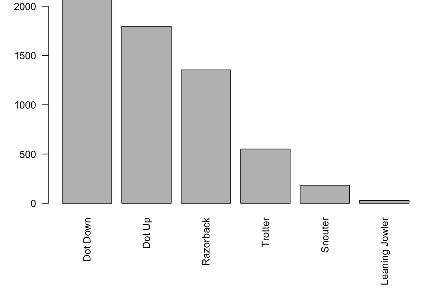
Figure 6.3: Frequency Bar Plot of Pig Rolls
While it is easy to see the relative differences of the outcomes above, using the proportions function will tell us the relative frequency of each outcome which will lead us towards the topic of this chapter, probability.
par( mar=c(8, 4, 0, 0) )
#The above is used to ensure that the names of the rolls are not cut off.
#The option `las = 2` is used to orient the names vertically.
barplot( sort( proportions( table( Pigs$black ) ), decreasing = T ), las =2 )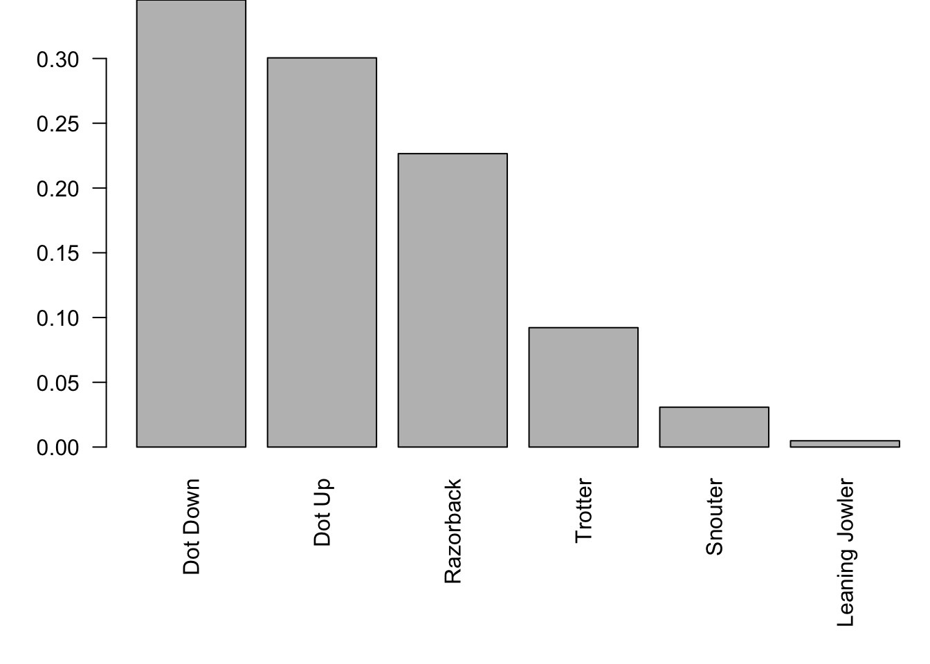
Figure 6.4: Relative Frequency Barplot of Pig Rolls
Now suppose you were handed the pig with the black dot on its snout and you wanted to know what the probability that the next roll would result in “Dot Up.”
Based on the barplot above, the proportion of the rolls in our dataset resulted in “Dot Up” was approximately 30%. However, is that the same as the probability of the next roll?64
The concepts of proportion and probability may be a bit intertwined for some readers and this is with good cause. Consider the following question.
This is asking the exact same thing as the following question.
That is, we can ask the same question about the proportion of things that are or ask about the probability that something will be.
In fact, once we have the Law of Large Numbers, Theorem 6.1, we will be able to say that after a large number of observations, it is basically impossible to distinguish between proportions and probabilities.
This setup was done to offer an example of a Probability Experiment before we formally defined it. We will now give the formal definition.
Definition 6.1 A Probability Experiment is the running of one or more Trials that each results in an Outcome. A collection of outcomes is called an Event and the collection of all outcomes is called the Sample Space. If \(E\) is an event, we use the notation \(P(E)\) to be the probability that a trial will result in the event \(E\).
We have attempted to make Definition 6.1 as readable as possible, but it is important to note that what we call an outcome cannot be made up of more than one possible result of the experiment. Outcomes are the simplest type of result from a probability experiment. As an example, the Ace of Hearts is an outcome while an Ace (of any suit) would be an event as it is made up of 4 different outcomes.
Example 6.1 The rolling of a single pig from the game of “Pass the Pigs” is an example of a probability experiment. In this case, we have
\[ S = \left\{ \text{Dot Up},\; \text{Dot Down},\; \text{Razorback},\; \text{Trotter},\; \text{Snouter},\; \text{Leaning Jowler} \right\}\] where each element of \(S\) is an outcome. An example of an event which is not an outcome would be what we can call a “Sider” which is either Dot Down or Dot Up. That is, formally, we would have
\[\text{Sider} = \left\{ \text{Dot Down},\; \text{Dot Up} \right\}.\]
While we do indeed have the notion of a probability experiment, we haven’t even mentioned the concept of probability which was also present in the definition. To get an idea of what rules probability should follow, we look at the properties that proportions follow. To get a quick feel, we can look at the proportions of the rolls for the black pig (rounded to 4 decimal places).
##
##  Dot Down    Dot Up Razorback   Trotter   Snouter   LJowler
##    0.3452    0.3005    0.2265    0.0922    0.0308    0.0049
It is clear that proportions should be values between 0 and 1 and that they should add up to 1. We use this as a basis to extend the definition of a probability experiment with what we call the Rules of Probability.
Definition 6.2 (The Rules of Probability) The probabilities of events in the sample space, \(S\), of a probability experiment must satisfy the following:
\(0 \leq P(E) \leq 1\) for all events \(E\).
\(P( a \text{ does not happen }) = 1 - P(a)\) for all outcomes \(a \in S\)
\(P(a \text{ or } b ) = P(a) + P(b)\) for all distinct outcomes \(a\) and \(b\)
If \(S\) is finite, \(\displaystyle{ \sum_{a \in S } P(a) = 1 }\) where \(a\) is taken over all outcomes in \(S\)
Example 6.2 We can fully realize the rolling of a pig as a probability experiment by assigning probabilities that satisfy Definition 6.2. Let the following table give the probability of \(P(a)\) for each of the outcomes \(a \in S\):
##
##  Dot Down    Dot Up Razorback   Trotter   Snouter   LJowler
##    0.3452    0.3005    0.2265    0.0922    0.0308    0.0049
Using the Rules of Probability, we can also find the following facts.
Each value in the table satisfies \(0 \leq P(a) \leq 1\)
\(P( \text{not a Razorback} ) = 1 - P(\text{Razorback}) = 1 - 0.2265 = 0.7735\)
\(P(\text{Sider}) = P(\text{Dot Down or Dot Up}) = P(\text{Dot Down}) + P(\text{Dot Up}) = 0.3452 + 0.3005\)
The very careful reader likely realized that we didn’t check that the sum of the probabilities was equal to 1. If you do check this, you will see that the probabilities is 1.0001. This is not a violation of Definition 6.2, but instead, just a consequence of us rounding rational numbers to only four decimal places. The following calculation shows that the sum of the probabilities would be 1 if we hadn’t rounded.
## [1] 16.2 Random Variables
Real world data displays variation among observations. As such, if we want to reasonably predict the behavior of data, we need to not only understand the most typical value it may take on, we must also understand how often it will take on other values. That is, we need to understand the probability that an observation takes on the possible values of the dataset. Because the values vary, we will look at how we can use the concept of a Random Variable to understand the variability in real world scenarios.
Definition 6.3 Given a probability experiment with a sample space, \(S\), we define a Random Variable, \(X\), to be a rule that assigns a real number to every outcome in \(S\). If \(S\) is already made up of real numbers, the rule is simply to let the random variable be equal to the outcome.
Example 6.3 In the case of Pass the Pigs, or rolling a single pig to be more precise, the random variable would be the following rule:
\[\begin{align*} \text{Dot Down} &\rightarrow 1\\ \text{Dot Up} &\rightarrow 2\\ \text{Razorback} &\rightarrow 3\\ \text{Trotter} &\rightarrow 4\\ \text{Snouter} &\rightarrow 5\\ \text{Leaning Jowler} &\rightarrow 6. \end{align*}\] We would now have the following facts about the new random variable:
\[\begin{align*} P(\text{Dot Down}) &= P( X =1)\\ P(\text{not a Trotter}) &= P(X \neq 4)\\ P(\text{Sider}) &= P(\text{Dot Down or Dot Up})\\ {} &= P(X = 1 \text{ or } X= 2) = P(X=1) + P(X=2) \end{align*}\]
Example 6.4 If we buy a two pound bag of potatoes, we could setup a probability experiment that counts the number of potatoes in the bag and let the random variable be the same number.
For any value, \(x_\emptyset\), that a random variable does not actually ever equal, we set \(P( X = x_\emptyset) = 0\).
Definition 6.4 A Discrete Random Variable is a random variable, \(X\), that takes on values among the whole numbers, \(\left\{ 0, 1, 2, 3, \ldots \right\}\).
We could define discrete random variables in a way to allow them to take on values in the negative integers or any other discrete65 set. However, mathematically, what we have done is equivalent and will allow us to keep discrete random variables in the realm of “counting” things.
Definition 6.5 Given a discrete random variable, \(X\), with possible outcomes given by \(S\), we can define the Population Mean of \(X\), denoted \(\mu_X\), to be
\[\mu_X = \sum_{x\in S} \big( x \cdot P(X = x)\big).\] We can further define the Population Standard Deviation of \(X\), denoted \(\sigma_X\), to be \[\sigma_X = \sqrt{\sum_{x\in S} \big( \left(x - \mu_X\right)^2 \cdot P(X = x)\big)}.\]
Like in Chapter 4, Definitions 4.8 and 4.9, we can define the Population Variance to be the square of the population standard deviation. In this case, we get the following: \[\sigma_X^2 = \displaystyle{\sum \left( \left(x - \mu_X\right)^2 \cdot P(X=x) \right)}.\]
The value \(\mu_X\) is sometimes called the Expected Value of \(X\) and denoted by \(E[X]\). We will illustrate the motivation behind this with Example 6.5.
Example 6.5 (Parameters of a Single Dice) Consider a “fair” 6-sided die, i.e. a die where \(P(X = n) = \frac{1}{6}\) for each \(n = 1,2, \ldots, 6\). We can calculate \(\mu_X\) and \(\sigma_X\) using Definition 6.5 as follows.
## [1] 1 2 3 4 5 6This gives us all the values of \(X\). As each probability is the same, we can simply multiply this vector by \(\frac{1}{6}\).
## [1] 0.1666667 0.3333333 0.5000000 0.6666667 0.8333333 1.0000000The last step is to simply find the sum of this new vector.
## [1] 3.5This says that the average roll of a die is 3.5. Of course, it is impossible to roll a 3.5, but if you rolled a large number66 of times, we expect that the average of all our rolls to be 3.5.
If we were playing a game where the value on the die was our score, we should expect to score 3.5 points with each roll. This is why we also call \(\mu_X\) the expected value.
We also note that the mean function built into R can do this immediately.
## [1] 3.5We can continue on to \(\sigma_X\) now that we have \(\mu_X = 3.5\). We first find the values of \((x - \mu_X)^2\).
## [1] 6.25 2.25 0.25 0.25 2.25 6.25We now multiply by \(\frac{1}{6}\) and then the square root of the sum to get \(\sigma_X\).
## [1] 1.707825One might expect this to match the sd function we introduced in Chapter 4, but that isn’t the case.
## [1] 1.870829The reason for this is the fact that sd measures the sample standard deviation and we want the population standard deviation. We need to use the formula given in Section 4.2.5. We can borrow the code used in Example 4.10 and get the following
## [1] 1.707825or we could use the function, popSD, that we developed then as well. [You may need to load the function using the “New Function” box found in Section 4.2.5.]
## [1] 1.707825This matches our manual calculation (and restores our faith in R). With a bit more care, we could workout that the exact representation of \(\sigma_X\) is \(\sqrt{\frac{35}{12}}\) which we “verify” by finding its approximation.
## [1] 1.707825Find the population mean and population standard deviation for a fair coin. That is, let
\[ \text{Heads} \rightarrow 1\] and \[ \text{Tails} \rightarrow 0.\] Assuming that \(P(X = 0) = P(X = 1) = \frac{1}{2}\), find \(\mu_X\) and \(\sigma_X\).
While “Pass the Pigs” provides a great look at asymmetric outcomes, it can still feel like a “game.” In the real world, we often encounter qualitative outcomes that we need to transform into numbers to make business or health decisions. This process of transformation is where the Random Variable truly shines.
A Random Variable is a function (a rule) that assigns a numeric value to every outcome in a sample space. We usually use a capital letter like \(X\) to represent the rule, and a lowercase \(x\) to represent the specific number it spits out.
Example 6.6 Imagine you are the manager of The Caffeine Statypus. Your customers don’t walk up to the counter and order “Outcome 1” or “Outcome 4.” They order drinks.
Before we can calculate a daily average or a standard deviation, we have to map our delicious drinks to numeric values. As we established in a Big Idea in Section 6.1, the world is full of qualitative “labels.” You can’t find the average of a Latte and a Muffin.
Suppose your Sample Space (\(S\)) consists of the four most common orders. We define the Random Variable \(X\) to be the number of syrup pumps in the drink.
| Outcome (\(s\)) | \(X(s)\) (Syrup Pumps) | \(P(X=x)\) |
|---|---|---|
| Drip Coffee | \(0\) | \(0.40\) |
| Vanilla Latte | \(3\) | \(0.30\) |
| Caramel Macchiato | \(4\) | \(0.20\) |
| Herbal Tea | \(0\) | \(0.10\) |
Note that the sum of the probabilities is \(1.00\), satisfying our Rules of Probability.
The manager wants to track the number of espresso shots in each drink as a new random variable, \(Y\).
- The Mapping: Define \(Y(\text{Drip Coffee}) = 0\), \(Y(\text{Vanilla Latte}) = 2\), and \(Y(\text{Herbal Tea}) = 0\).
- The “Missing” Link: We also know a Caramel Macchiato has \(2\) shots. Using the probabilities from the table above, find \(P(Y=2)\).
- Logic Check: Why is \(P(Y=2)\) the sum of the probabilities for the Latte and the Macchiato? (Hint: See the mapping rule in Definition 6.3.)
- Extension: Find the expected value of \(Y\).
6.3 The Law of Large Numbers
In Section 6.1, we defined the probability of the different outcomes for rolling a pig based off of six thousand actual rolls67 of a little physical pig. This is tied to what is called the Frequentist View of Probability where we look at probabilities as the relative frequency that events happen over the long run. This likely contrasts to the types of probabilities you may have studied before where we simply assumed that “all outcomes are equally likely” in cases such as flipping a coin or rolling a standard six-sided die. Outside of a classroom, it is unlikely to be able to have much confidence that any situation is perfect enough to assume that “all outcomes are equally likely” and we are better off looking at what happens over the long run in a large number of trials.
Theorem 6.1 (Law of Large Numbers) The Law of Large Numbers, which we will abbreviate as the LLN, states that the observed relative frequency of an event may not equal the true probability over a small number of trials. However, as the number of trials increases, the relative frequency of an event will68 get closer and closer to the true probability.
In situations like a coin, we have a theoretical probability that we can use the LLN to compare to observed relative frequencies. However, in the case of situations like Pass the Pigs, we do not have any sense of how to find a theoretical value of \(P(\text{Trotter})\). However, we can use the Law of Large Numbers to actually get an estimate of the “true” probability of a Trotter. That is to say, if we use a large number of trials, we can assume that the observed relative frequency of an outcome is close to its true probability.69
What the Law of Large Number is loosely saying is that if we are looking at a large number of observations that the observed proportions and the “true” probabilities are basically the same. In fact, we can use a large number of observations to determine an estimate of a “true” probability if we are unable to find it with other techniques.
This means that the probabilities we defined for the pigs in Example 6.2 were indeed good estimates of the “unknowable true probabilities” of each outcome for rolling a pig.
Thus, to get a good estimate of a probability where we do not have a theoretical understanding of, we simply need to repeat the experiment a large number of times. While practical experiments such as the six thousand rolls of a pig are tangible and understandable, they are time consuming human beings are prone to recording errors over such a large number of trials. However, the rise of computational power now allows us to do repeated trials of some probability experiments with the precision and repeatability of a machine.
Definition 6.6 A Simulation is the use of computers to run theoretical trials of a probability experiment.
This exploration is a Simulation to support the Law of Large Numbers. It shows the result of flipping a fair coin 100 times and the running proportion of the number of heads as each flip occurs.
If you haven’t adjusted the “Randomizer,” you should see that the sequence of flips began with 5 straight heads. This initial start may make you think the coin is unfair, but we see as the coin was flipped more and more, the proportion approaches the central red line which shows the “theoretical” or true probability a fair coin should achieve.
In the default setting of the “Style” switch, the blue region shows an error up to 2%, the orange region has an error of 2% to 5%, and the purple region shows an error up to 10%. If you toggle the Style switch, you get the region within one, two, and three standard deviations of the theoretical populations. This topic is further studied in Chapter 9. You can also see Section 7.5 for an idea of what the colored regions represent in the alternate style.
Feel free to slide the “Randomizer” around to see other samples of random coin flips and watch how the proportions do appear to “settle in” towards the red line.
If you want to play with this graph even more, click on the “edit graph on desmos” graphic in the lower right corner of the window. There you can find some even more advanced controls that were not easily adapted to an embedded visualization.
Example 6.7 In Example 6.5, we used Definition 6.5 to find the population mean and standard deviation of mean value of rolling a fair dice. There we found that \(\mu_X = 3.5\) and we claimed that \(\sigma_X = \sqrt{\frac{35}{12}}\) while showing that it was numerically approximately \(1.707825\).
To test this, we could simply roll a fair dice a large number of times and calculate the mean and standard deviation. However, if we wanted to get a really good estimate, then we should be using a truly large number of trials, say one million. It is highly unlikely that anyone has the time to roll and record the result of one million dice rolls.70
However, it is clear that computers can greatly expedite this endeavor. To do this, we need to revisit the sample() function we first encountered in Chapter 2.
The syntax of sample we will now use is
where the arguments are:
x: The vector of elements from which you are sampling.size: The number of samples you wish to take.replace: Whether you are sampling with replacement or not. Sampling without replacement means that sample will not pick the same value twice, and this is the default behavior. Passreplace = TRUEto sample if you wish to sample with replacement.prob: A vector of probabilities or weights associated withx. It should be a vector of non-negative numbers of the same length asx.
If the sum of prob is not 1, it will be normalized. That is, each value in prob will be taken to be out of the sum of prob. For example, if the values in prob were 0.2, 0.3, and 0.4, then the actual probabilities would be 0.2/0.9 = 2/9, 0.3/0.9 = 1/3, and 0.4/0.9 = 4/9. If prob is not provided, then each element of x is considered to be equally likely.
Also, recall that sample() does invoke a “random” element so that it will vary each time you run the function. As such, if you run the code shown on the screen on your own machine, it is highly unlikely that it will match what you see here or the results of anyone else making the calculations.
Example 6.8 Thus, if we want to simulate the rolling of one million dice, we have to establish the values of the arguments: x, size, and replace. Due to the remark above, we can omit the argument prob as we will be assuming that the probability of each outcome is equal.
The value of x should be the sample space we are sampling from. In this case, it should be the numbers \({1,2,3,4,5,\text{and }6}\). We can do this by setting x to be 1:6. We verify this by simply asking R to spit out the result of 1:6.
## [1] 1 2 3 4 5 6The size argument is pretty straight forward and we will use size = 1000000. Here is where our use of sample will differ from Chapter 2. There we never invoked the replace argument as we didn’t want to include any individual in a sample more than once. However, if we were to do that now, we would run into problems as we are certain to get duplicates of some values of a dice if we roll it more than 6 times. Setting replace = TRUE means that we “pull” a value from x and then “put it back” leaving x the same for each time it selects a value.
Putting it all together, we get the following line of code where we will save our result as the vector called rolls.
To see the result of this, we can use the head() function which we introduced in Chapter 1.
## [1] 4 3 4 5 2 6This tells us that R simulated rolling a dice and observed a 4 and then a 3 and then another 4. If we had not set replace = TRUE, this would not be possible. We can now use the Code Template from Section 3.3.2 to look at the histogram of this discrete data.
#Data must be supplied
data <- rolls
#Value must be given
bin_width <- 1
#Do not change any values below this comment
hist(
      data,
      freq = TRUE,
      breaks = seq(
                      from = min( data, na.rm = TRUE ) - 0.5,
                      to = max( data, na.rm = TRUE ) + bin_width - 0.5,
                      by = bin_width
                  )
    )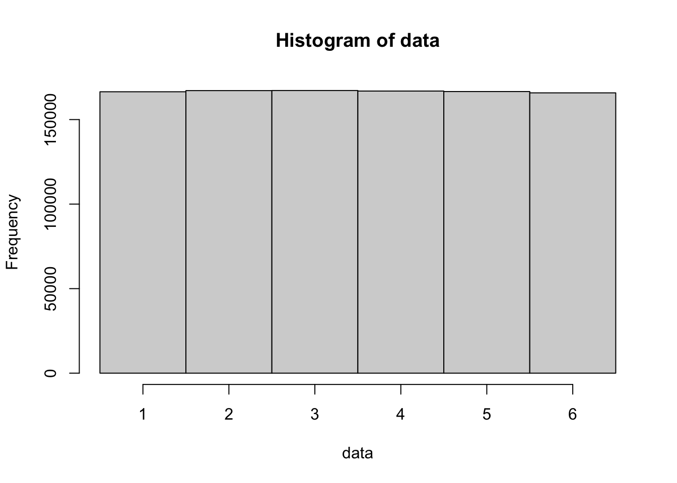
This shows a nearly perfect uniform distribution of values from 1 to 6 as we would expect from one million rolls of a fair dice. We will look at just how realistic this is in Chapter 9 when we investigate “precision dice.”
Being that our sample appears to be a very good estimation of a theoretically “fair” dice, we can simply ask R to calculate the mean of rolls and compare it to the theoretical value of 3.5.
## [1] 3.497402This estimate is really good being off by less than 3 thousandths. This gives us confidence to calculate the standard deviation as well.
## [1] 1.706123This is also very consistent with the value of \(1.707825\) we found in Example 6.5. Now, the astute reader may be crying foul right now saying that Definition 6.5 was for the population standard deviation and we know that sd calculates the sample standard deviation. As we mentioned in Chapter 4, we can convert from a sample standard deviation to the population standard deviation by multiplying by \(\sqrt{\frac{n-1}{n}}\) where \(n\) is the size of the sample. In our case, \(n\) is one million and we get that \(\sqrt{\frac{n-1}{n}} = \sqrt{\frac{999999}{1000000}} \approx 0.9999995\). We could also load the popSD function introduced in Section 4.2.5 and then run it on rolls as shown below.
## [1] 1.706122This shows that the sample standard deviation and the population standard deviation only differ (by 1) in the one millionths place! Thus, it is unnecessary to concern ourselves with the difference as we do not expect our estimate to be that close.
This example can be viewed in one of two ways.
We can take this example as a simulation which confirms the calculations made in Example 6.5.
We could take the results of this example as our estimates of \(\mu_X\) and \(\sigma_X\) pretending we didn’t know the formulas of Definition 6.5 and trusting that the results are close to the true (and possibly unknown) values via the Law of Large Numbers, Theorem 6.1.
Example 6.9 (Coding the Coffee) Here we will revisit The Caffeine Statypus, we first saw in Example 6.6. In R, once we have assigned our numeric values (our mapping), we can simulate a day at the shop using the sample function by invoking the prob argument. To simulate the total amount of syrup used for the next 50 customers at The Caffeine Statypus, we use the following blocks of code.
This sets the values of the 4 different outcomes: Drip Coffee, Vanilla Latte, Caramel Macchiato, and Herbal Tea. We now define the probabilities associated with those values.
We can now simulate 50 customers via the following exploded code chunk.
With this, we can ask a variety of questions. For example, “what was the total number of syrup pumps for these 50 people?” This is easily done with the sum function.
## [1] 86Notice that in the code above, R doesn’t care that 2.50 represents a “Drip Coffee.” By the time we reach the simulation stage, we have already completed the mapping. This is why the definition of a Random Variable is a powerful “bridge” in statistics.
Find \(E[X]\) for the random variable, \(X\) as defined in Example 6.9
Give a practical interpretation of this value and how the manager may use it for planning purposes.
6.4 Continuous Probabilities
Thus far, all of the random variables that we have worked with have been Discrete Random Variables. We now move on to where the random variable can take on values across a continuous region of the real line.
Definition 6.7 If a random variable can take on any value inside a continuous interval \((a,b)\) inside the real numbers, then we call it a Continuous Random Variable. We require that
\[P( X= x_0 ) = 0\] for any value \(x_0\in (a,b)\). The fact that the probability of equaling any given value is zero is what we call the Continuous Variable Axiom.
The restriction that \(P(X = x_0) = 0\) will ensure that the Distribution Function we define in Section 6.5.2 will be continuous as long as \(X\) is a continuous random variable.
According to Snickers.com, as of early 2025, the weight of a Snickers bar in the United States is 1.86 ounces. However, it is not possible to produce physical bars that are exactly 1.86 ounces nor is it possible to produce bars which have identical weights if we measure to a high enough level of precision. To understand the distribution of weights of Snickers bars, we will use the vector Snickers which contains the weight of 100 Snickers bars.
The reader can see Section 6.7.2 to get more information about this dataset.
Snickers <- c(
51.1, 53.8, 51.1, 53.8, 51.9, 52.5, 53.2, 53.8, 52.4, 54.0,
53.5, 54.4, 51.1, 52.4, 50.8, 52.1, 51.9, 51.2, 52.7, 53.3,
52.1, 54.1, 52.7, 54.1, 51.9, 53.7, 52.2, 53.7, 54.2, 52.2,
52.5, 54.5, 53.0, 51.9, 54.4, 54.7, 53.0, 53.8, 54.3, 53.3,
52.4, 51.2, 53.5, 52.4, 52.3, 55.2, 51.2, 54.3, 53.3, 51.9,
51.3, 53.8, 53.3, 52.0, 50.3, 51.8, 51.1, 52.6, 52.5, 53.9,
53.1, 53.9, 52.9, 52.2, 50.5, 52.5, 50.3, 52.2, 52.2, 51.7,
52.0, 52.5, 53.1, 53.8, 54.0, 53.4, 52.3, 50.9, 53.9, 53.4,
53.4, 52.5, 53.6, 53.0, 56.2, 54.2, 52.5, 52.4, 53.3, 52.9,
51.8, 50.9, 52.3, 54.0, 51.2, 53.6, 51.1, 50.3, 53.2, 52.6
)/28.35
We can look at the first few values of Snickers using head.
## [1] 1.802469 1.897707 1.802469 1.897707 1.830688 1.851852We can also run summary on Snickers to get a quick look at some of the numerical summaries of our data.
##    Min. 1st Qu.  Median    Mean 3rd Qu.    Max.
##   1.774   1.833   1.855   1.860   1.894   1.982
We see that our data gives a mean right at 1.86 ounces.
Construct a boxplot of Snickers and discuss what type of skew you see in the data. Does the skew seem to favor the consumer or the manufacturer?
We continue on with our analysis of Snickers by looking at a histogram.
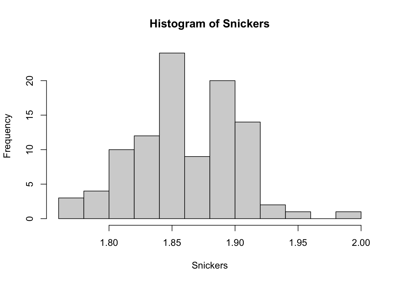
Figure 6.5: Frequency Histogram of Snickers Bar Weights (oz)
Here we saved hist( Snickers ) as SnickersHist which will allow us to extract more information from Snickers than just the plot we see above. By default, hist returns a list of six different variables. The curious reader can examine this in more detail by looking at ?hist and scrolling down to the Value section of the help file.
For discrete data, the area of the bars in a relative frequency histogram was equivalent to the proportion. Let’s pull out the frequencies of each bin to find the area of the boxes in our histogram
## [1] 3 4 10 12 24 9 20 14 2 1 0 1To get the areas of the boxes, we need to know precisely how wide the bins are. We can find this by looking at the boundary of the bins using the breaks column of SnickersHist.
## [1] 1.76 1.78 1.80 1.82 1.84 1.86 1.88 1.90 1.92 1.94 1.96 1.98 2.00Thus, the areas of the boxes can be found by multiplying the frequencies, which is contained in SnickersHist$counts, by the width of each bin which is 0.02.
## [1] 0.06 0.08 0.20 0.24 0.48 0.18 0.40 0.28 0.04 0.02 0.00 0.02To compare our histogram to the area idea we developed from discrete bar plots, we find the sum of the areas of the rectangles.
## [1] 2To make the setup match what we had with the pigs in Section 6.1 we would want to not use the counts, but the counts divided by exactly 2 so that this sum would be 1 so that we can be consistent with Definition 6.2.
If we set freq = FALSE in hist, this is exactly what the values on the vertical axis are!
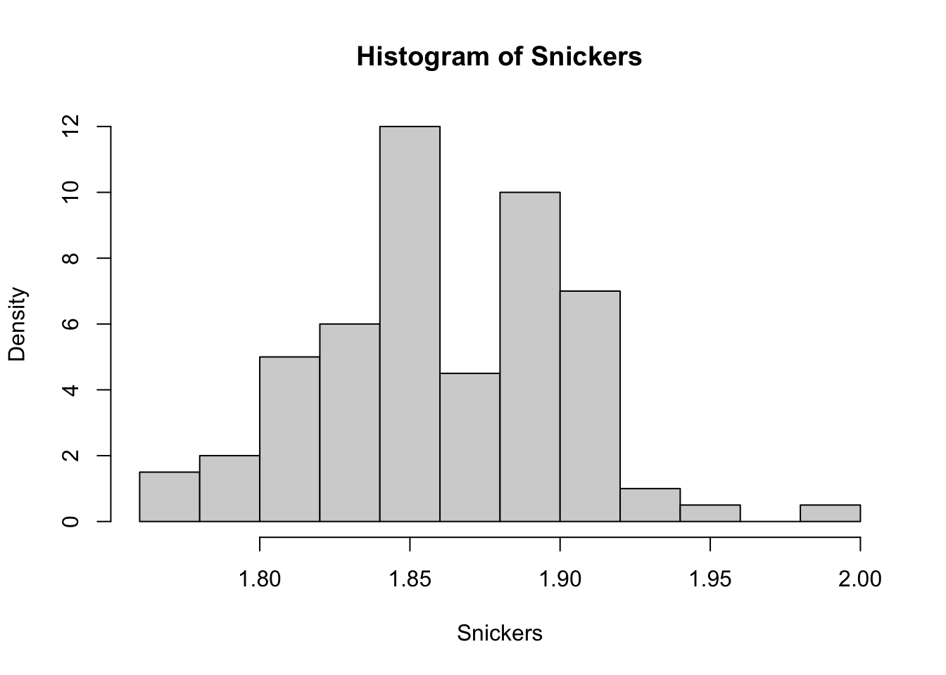
Figure 6.6: Density Histogram of Snickers Bar Weights (oz)
Thus what R is labeling as Density in Figure 6.6 is the height of the box needed so that the proportion of values in the bin is equal to the area of the box. This leads us to our definition of Density in the case of a histogram.
Definition 6.8 The Density of a histogram bin is the height such that the area of the rectangle is equal to the proportion of values that fall within that bin.
The careful reader will likely wonder about using histograms for discrete values in Section 6.1 instead of bar plots when the data could be viewed as numeric via the assignments we made in Example 6.3. We will require that discrete random variables take on integer values so that the bins will have width of 1 like we setup in Section 3.3.2. This will ensure that the height of each rectangle is equal to its area so that that density and proportion are interchangeable.
We can also find the densities of a histogram directly using the density column of a saved histogram like below.
## [1] 1.5 2.0 5.0 6.0 12.0 4.5 10.0 7.0 1.0 0.5 0.0 0.56.5 Probability Functions
As we get towards the end of this chapter, we want to establish the structure we will use with random variables. These functions will allow us to use random variables to analyze and understand probability questions as well as lead us towards being able to make inferences about a population based on the statistics we have from a sample.
6.5.1 Density Function
In Section 6.4, we defined density in terms of a bin in a histogram. It is the goal of this section to define it for each value that a random variable can take. If we have a discrete random variable, the remark at the end of Section 6.4 means we can simply define the density of a discrete random variable to be the density we defined for the bin of width 1 as we setup in Section 3.3.2.
This leads us to the idea of assigning the density of a bin to the midpoint of the bin, but this only allows us to define it for a number of values of the data equal to the number of bins in the histogram. Thus, to define density for more values, we need to have histograms with more bins, a lot more bins.
To be able to get meaningful information from a histogram with a lot of bins, we need a lot more bars than one hundred. We will look at the histogram of a sample of one hundred thousand Snickers bars.71 We start with an artificially small number of bins.
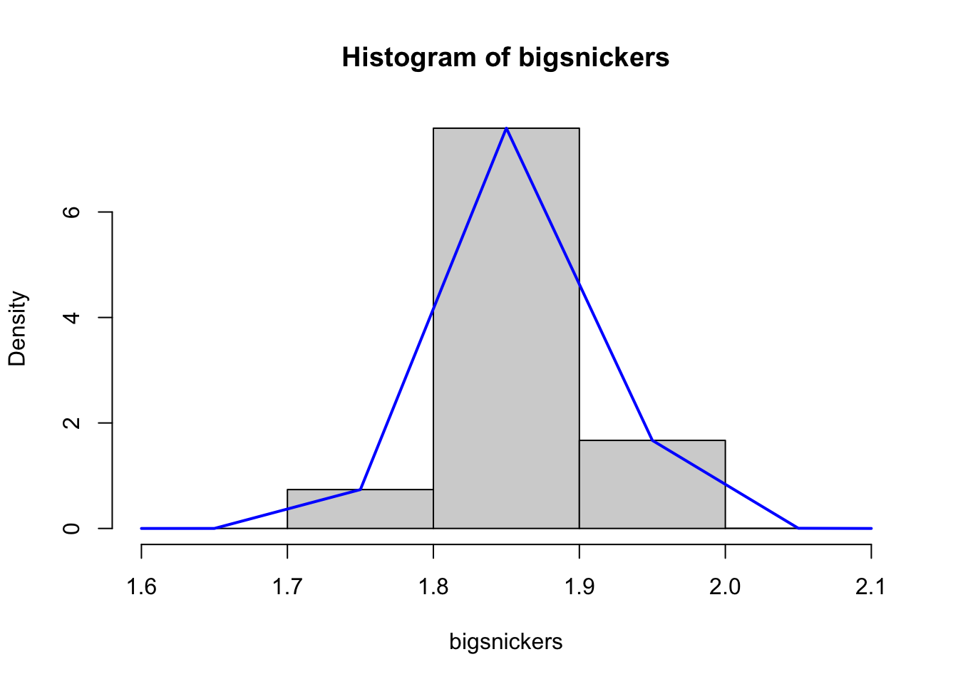
Figure 6.7: Density Histograms of Snickers Bar Weights with 5 Bins
The blue curve72 on top of the histogram is created by connecting the top of each rectangle at the midpoint of each bin. This means that the blue curve can be taken as a function which defines the density for all of the values in the range of the histogram. However, as we mentioned, the number of bins in Figure 6.7 was artificially set to be low, only 5 in this case.
If we increase the number of bins to only 8, we get the following plot.
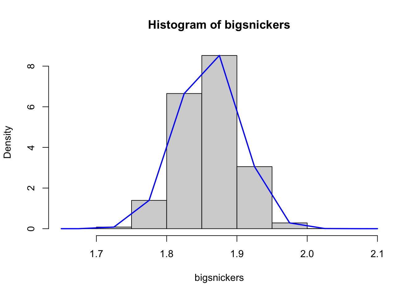
Figure 6.8: Density Histograms of Snickers Bar Weights with 8 Bins
If we again view the blue curve as the density function, we see that we are getting more detail in the curve and that it would give more “correct values” (i.e. that match the histogram) since there are more bins.
Naturally, we can increase the number of bins even further, this time to 18.
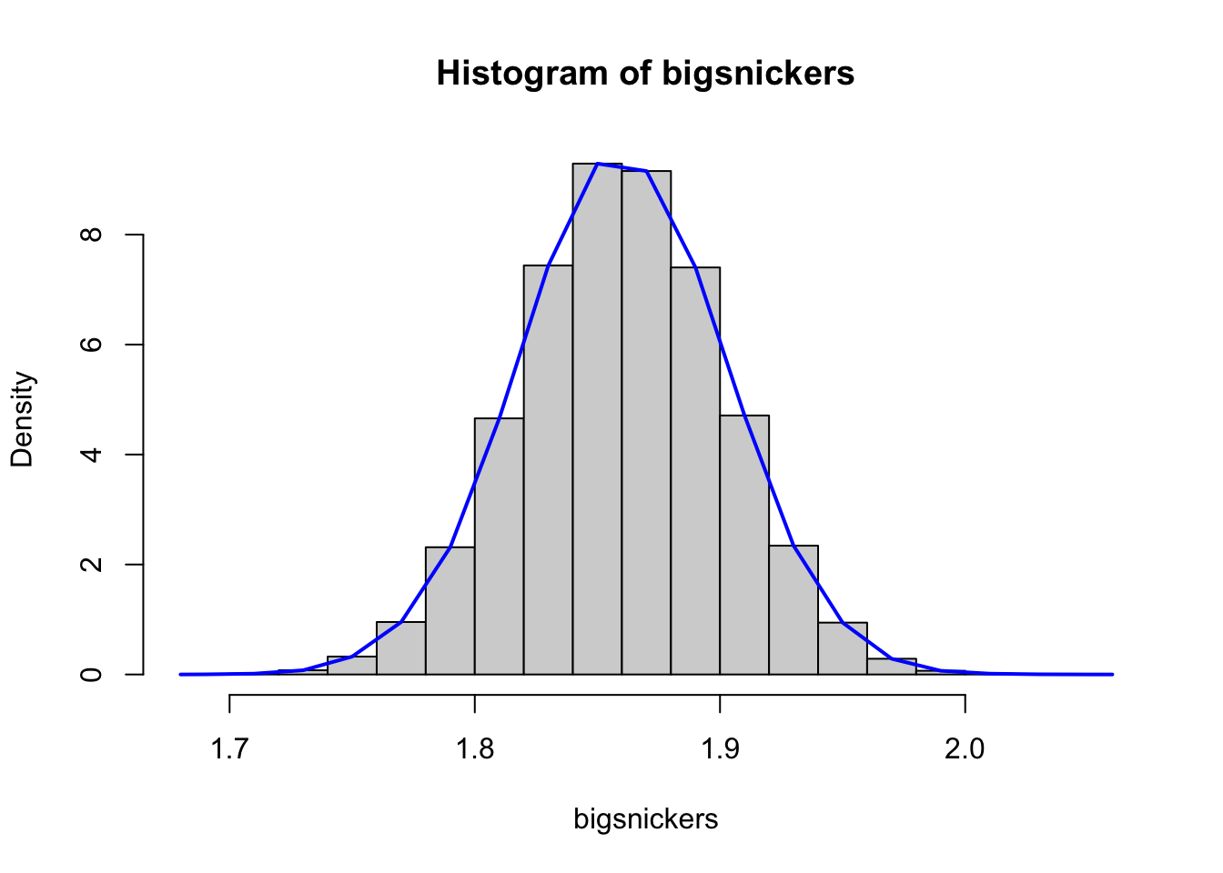
Figure 6.9: Density Histograms of Snickers Bar Weights with 18 Bins
The blue curve in Figure 6.9 is starting to actually look a true “curve” in the more basic sense of the word.
As we increase the number of bins in a histogram, the density “polygon” we have been creating appears to be approaching a smooth curve.
Cranking up the number of bins to 68 gives the following plot.
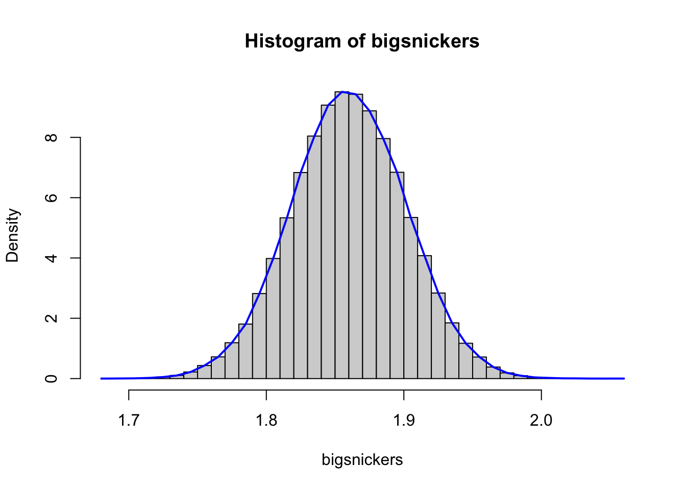
Figure 6.10: Density Histograms of Snickers Bar Weights with 68 Bins
Figure 6.10 looks like a smooth curve at first glance, but if one looks very closely at it, especially near the middle of the values, it can be seen to still be made up of straight line segments.
This concept can continue to get a function which is “correct” at as many points as we wish as long as we have enough data values in our histogram. Imagining the possibility of making a histogram of an infinite number of Snickers bars using an infinite number of bins would yield a curve that looks like the following.
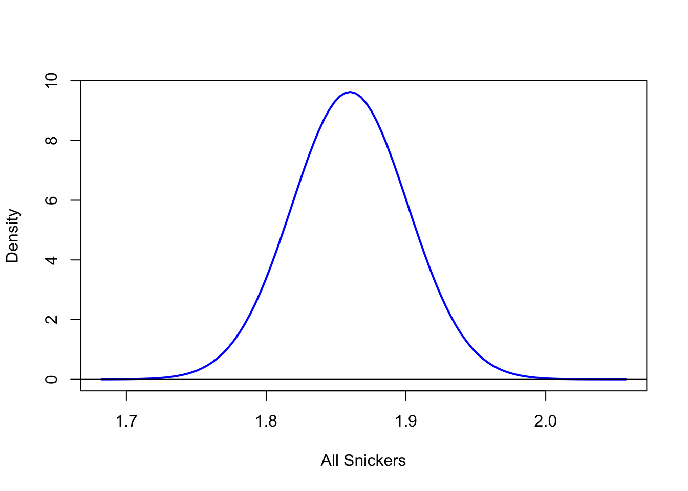
Figure 6.11: Density Function of Snickers Bars
Being that each histogram in Figures 6.7 to 6.10 was defined to have a total area of 1 when we add the area of the rectangles, we get that the area bound by the blue curve and the \(x\)-axis is 1 as well. This leads us to the definition of a Density Function.
Definition 6.9 Given a random variable that can take on any value on a continuous interval of the real line, we define the Density Function of a Continuous Random Variable to be the function that results from using the technique outlined above between Figures 6.7 to 6.10 and resulting in a graph like seen in Figure 6.11. If this function is called \(\text{ddist}\), then we demand it satisfy the following:
- \(\text{ddist}(x) \geq 0\) for all values of \(x\).
- The area under the graph of \(\text{ddist}(x)\) is equal to 173.
- \(P( a < X \leq b)\) is the area under the curve, \(y = \text{ddist}(x)\), between \(x=a\) and \(x=b\).
To understand the density of a continuous random variable, we can use the following Desmos exploration.
If you change the values of \(a\) and \(b\) by dragging the points along the \(x\)-axis, we get a new probability of form \(P(a < X\leq b)\).
For completeness, we will give a different definition of a Density Function for a discrete random variable.
Definition 6.10 Given a random variable that can take values within a subset of the integers, we define the Density Function of a Discrete Random Variable to be a function, \(\text{ddist}\), that satisfies the following:
- \(P( X = x_0 ) = \text{ddist}( x_0 )\) for all integers \(x_0\).
- \(\text{ddist}(x) \geq 0\) for all values of \(x\).
- \(\sum \text{ddist}(x_i) = 1\) where the sum is taken over all integers, \(x_i\).
6.5.2 Distribution Function
The density function above makes it easy to define what we will call the Distribution Function.
Definition 6.11 Given a random variable, \(X\), we define the Distribution Function of it to be a function \(\text{pdist}\) that satisfies
\[\text{pdist}(q )= P(X \leq q)\] for any real number \(q\)
It is important to note that we will not show any graphs of distribution functions or the quantile functions we define in Section 6.5.3. All of the graphs shown in this book are the graphs of density functions. However, we will learn how to interpret the distribution and quantile functions based off of density graphs.74
We can explore a generic distribution function using the Desmos exploration below which you can interact with.
Feel free to play around with it and then watch the following video walking through it.
6.5.3 Quantile Function
Due to the exploration we just looked at, we can see that there is a one to one correspondence between the quantiles and the probabilities. This leads us to consider the inverse function of \(\text{pdist}\).
Definition 6.12 Given a random variable, \(X\), with a distribution function, \(\text{pdist}\), we define the variable’s Quantile Function to be a function \(\text{qdist}\) defined by
\[\text{qdist}( p ) = \text{pdist}^{-1} (p).\]
There can be some issues with Definition 6.12 if there is any open interval where \(\text{ddist}\) is constant 0 for a continuous random variable. There can also be some trickiness in defining the quantile function for discrete random variables as only discrete values of probabilities are actually possible. Fortunately, these issues will not cause us much concern and we can use the above as our definitions. For example, you can see the remark in Section 8.2.3 that discusses how the function qbinom() handles this situation for the discrete Binomial distribution.
We can explore a generic quantile function using the Desmos exploration below which you can interact with.
Feel free to play around with it and then watch the following video walking through it.
6.5.4 Random Function
We saw in Section 6.3 that simulations can offer a great way to run probability experiments. If we want to run probability experiments that can be modeled by random variables, we need a function that can generate random values of the variable.
Definition 6.13 Given a random variable, \(X\), with a density function, \(\text{ddist}\), we define the variable’s Random Generation Function to be a function \(\text{rdist}\) that generates values that \(X\) takes on. A large number of values obtained from \(\text{rdist}\) will yield a histogram which can be closely modeled by \(\text{ddist}\).
The concept of a Random Generation Function is only necessary when running simulations. This concept may not be covered in some courses using this text.
6.6 Mind Your p’s and q’s75
Keeping pdist and qdist straight can be difficult for new users. It can be helpful to think of the p being “probability”( or proportion) and q being “quantile”. So pdist is the function that has an output of p and qdist is the function that has an output of q.
Another way to think of it is that you put a p into qdist to get a q or inversely we put a q into pdist to get a p.
Review the explorations in Sections 6.5.2 and 6.5.3 if you are struggling to mind your ps and qs.
Review for Chapter 6
Chapter 6 Quiz: From Proportions to Probabilities
This quiz tests your understanding of core concepts in probability, random variables, and the rules governing probability calculations presented in Chapter 6. The answers can be found prior to the Exercises section.
- True or False: The Law of Large Numbers (LLN) states that as the number of trials in a probability experiment increases, the observed relative frequency of an event will get closer and closer to the true probability.
- True or False: The Frequentist View of Probability looks at probabilities as the relative frequency that events happen over the long run.
- True or False: A simulation is defined as the use of computers to run theoretical trials of a probability experiment.
- True or False: The quantile function, \(\text{qdist}\), is used to find the cumulative probability (the area under the curve) up to a specified value of the random variable.
- True or False: The density function, \(\text{ddist}\), is the most useful function for directly calculating probabilities for a continuous random variable because \(P(X=x_0)\) is the value of this function.
- True or False: The sample space is a list of all possible outcomes of a probability experiment.
- True or False: The Law of Large Numbers suggests that if you flip a fair coin and observe 9 heads in a row, the probability of the next flip being tails is greater than \(0.5\) to balance the prior results.
- True or False: For a continuous random variable, the probability of the variable equaling any single given value, \(P(X=x_0)\), is defined to be zero.
- True or False: A random variable must always be a discrete variable, as it represents counts of outcomes from a probability experiment.
- True or False: If a computer function \(\text{rdist}\) generates values for a random variable, a large number of generated values will produce a histogram that can be closely modeled by the variable’s density function, \(\text{ddist}\).
Definitions
Section 6.1
Definition 6.1 \(\;\) A Probability Experiment is the running of one or more Trials that each results in an Outcome. A collection of outcomes is called an Event and the collection of all outcomes is called the Sample Space. If \(E\) is an event, we use the notation \(P(E)\) to be the probability that a trial will result in the event \(E\).
Definition 6.2: The Rules of Probability \(\;\) The probabilities of events in the sample space, \(S\), of a probability experiment must satisfy the following:
\(0 \leq P(E) \leq 1\) for all events \(E\).
\(P( a \text{ does not happen }) = 1 - P(a)\) for all outcomes \(a \in S\)
\(P(a \text{ or } b ) = P(a) + P(b)\) for all distinct outcomes \(a\) and \(b\)
If \(S\) is finite, \(\displaystyle{ \sum_{a \in S } P(a) = 1 }\) where \(a\) is taken over all outcomes in \(S\)
Section 6.2
Definition 6.3 \(\;\) Given a probability experiment with a sample space, \(S\), we define a Random Variable, \(X\), to be a rule that assigns a real number to every outcome in \(S\). If \(S\) is already made up of real numbers, the rule is simply to let the random variable be equal to the outcome.
Definition 6.4 \(\;\) A Discrete Random Variable is a random variable, \(X\), that takes on values among the whole numbers, \(\left\{ 0, 1, 2, 3, \ldots \right\}\).
Definition 6.5 \(\;\) Given a discrete random variable, \(X\), with possible outcomes given by \(S\), we can define the Population Mean of \(X\), denoted \(\mu_X\), to be
\[\mu_X = \sum_{x\in S} \big( x \cdot P(X = x)\big).\] We can further define the Population Standard Deviation of \(X\), denoted \(\sigma_X\), to be \[\sigma_X = \sqrt{\sum_{x\in S} \big( \left(x - \mu_X\right)^2 \cdot P(X = x)\big)}.\]
Like in Chapter 4, we can define the Population Variance to be the square of the population standard deviation. In this case, we get the following: \[\sigma_X^2 = \displaystyle{\sum \left( \left(x - \mu_X\right)^2 \cdot P(X=x) \right)}.\]
Section 6.3
Definition 6.6 \(\;\) A Simulation is the use of computers to run theoretical trials of a probability experiment.
Section 6.4
Definition 6.7 \(\;\) If a random variable can take on any value inside a continuous interval \((a,b)\) inside the real numbers, then we call it a Continuous Random Variable. We require that
\[P( X= x_0 ) = 0\] for any value \(x_0\in (a,b)\). The fact that the probability of equaling any given value is zero is what we call the Continuous Variable Axiom.
Definition 6.8 \(\;\) The Density of a histogram bin is the height such that the area of the rectangle is equal to the proportion of values that fall within that bin.
Section 6.5
Definition 6.9 \(\;\) Given a random variable that can take on any value on a continuous interval of the real line, we define the Density Function of a Continuous Random Variable to be the function that results from using the technique outlined above between Figures 6.7 to 6.10 and resulting in a graph like seen in Figure 6.11. If this function is called \(\text{ddist}\), then we demand it satisfy the following:
- \(\text{ddist}\) is a continuous function
- \(\text{ddist}(x) \geq 0\) for all values of \(x\).
- The area under the graph of \(\text{ddist}(x)\) is equal to 176.
- \(P( a < X \leq b)\) is the area under the curve, \(y = \text{ddist}(x)\), between \(x=a\) and \(x=b\).
Definition 6.10 \(\;\) Given a random variable that can take values within a subset of the integers, we define the Density Function of a Discrete Random Variable to be a function, \(\text{ddist}\), that satisfies the following:
- \(P( X = x_0 ) = \text{ddist}( x_0 )\) for all integers \(x_0\).
- \(\text{ddist}(x) \geq 0\) for all values of \(x\).
- \(\sum \text{ddist}(x_i) = 1\) where the sum is taken over all integers, \(x_i\).
Definition 6.11 \(\;\) Given a random variable, \(X\), we define the Distribution Function of it to be a function \(\text{pdist}\) that satisfies
\[\text{pdist}(q )= P(X \leq q)\] for any real number \(q\)
Definition 6.12 \(\;\) Given a random variable, \(X\), with a distribution function, \(\text{pdist}\), we define the variable’s Quantile Function to be a function \(\text{qdist}()\) defined by
\[\text{qdist}( p ) = \text{pdist}^{-1} (p).\]
Definition 6.13 \(\;\) Given a random variable, \(X\), with a density function, \(\text{ddist}\), we define the variable’s Random Generation Function to be a function \(\text{rdist}\) that generates values that \(X\) takes on. A large number of values obtained from \(\text{rdist}\) will yield a histogram which can be closely modeled by \(\text{ddist}\).
Results
Section 6.3
Theorem 6.1: Law of Large Numbers \(\;\) The Law of Large Numbers, which we will abbreviate as the LLN, states that the observed relative frequency of an event may not equal the true probability over a small number of trials. However, as the number of trials increases, the relative frequency of an event will77 get closer and closer to the true probability.
Big Ideas
Section 6.1
The concepts of proportion and probability may be a bit intertwined for some readers and this is with good cause. Consider the following question.
This is asking the exact same thing as the following question.
That is, we can ask the same question about the proportion of things that are or ask about the probability that something will be.
In fact, once we have the Law of Large Numbers, Theorem 6.1, we will be able to say that after a large number of observations, it is basically impossible to distinguish between proportions and probabilities.
Section 6.2
A Random Variable is a function (a rule) that assigns a numeric value to every outcome in a sample space. We usually use a capital letter like \(X\) to represent the rule, and a lowercase \(x\) to represent the specific number it spits out.
Section 6.3
What the Law of Large Number is loosely saying is that if we are looking at a large number of observations that the observed proportions and the “true” probabilities are basically the same. In fact, we can use a large number of observations to determine an estimate of a “true” probability if we are unable to find it with other techniques.
This means that the probabilities we defined for the pigs in Example 6.2 were indeed good estimates of the “unknowable true probabilities” of each outcome for rolling a pig.
As we increase the number of bins in a histogram, the density “polygon” we have been creating appears to be approaching a smooth curve.
Important Alerts
Section 6.3
It is important to note that we will not show any graphs of distribution functions or the quantile functions we define in Section 6.5.3. All of the graphs shown in this book are the graphs of density functions. However, we will learn how to interpret the distribution and quantile functions based off of density graphs.78
Important Remarks
Section 6.1
We have attempted to make Definition 6.1 as readable as possible, but it is important to note that what we call an outcome cannot be made up of more than one possible result of the experiment. Outcomes are the simplest type of result from a probability experiment. As an example, the Ace of Hearts is an outcome while an Ace (of any suit) would be an event as it is made up of 4 different outcomes.
Section 6.2
For any value, \(x_\emptyset\), that a random variable does not actually ever equal, we set \(P( X = x_\emptyset) = 0\).
We could define discrete random variables in a way to allow them to take on values in the negative integers or any other discrete79 set. However, mathematically, what we have done is equivalent and will allow us to keep discrete random variables in the realm of “counting” things.
The value \(\mu_X\) is sometimes called the Expected Value of \(X\) and denoted by \(E[X]\). We will illustrate the motivation behind this with Example 6.5.
Section 6.5
The restriction that \(P(X = x_0) = 0\) will ensure that the Distribution Function we define in Section 6.5.2 will be continuous as long as \(X\) is a continuous random variable.
The careful reader will likely wonder about using histograms for discrete values in Section 6.1 instead of bar plots when the data was numeric. We will require that discrete random variables take on integer values so that the bins will have width of 1 like we setup in Section 3.3.2. This will ensure that the height of each rectangle is equal to its area so that that density and proportion are interchangeable.
Definition 6.10 does allow for \(\text{ddist}\) to be defined for more values than just the integers so that we can view it as the “tops” of a histogram as seen in Section 3.3.2.
There can be some issues with Definition 6.12 if there is any open interval where \(\text{ddist}\) is constant 0 for a continuous random variable. There can also be some trickiness in defining the quantile function for discrete random variables as only discrete values of probabilities are actually possible. Fortunately, these issues will not cause us much concern and we can use the above as our definitions.
New Functions
Section 6.3
The syntax of sample we will now use is
#This code will not run unless the necessary values are inputted.
sample( x , size , replace , prob )
where the arguments are:
x: The vector of elements from which you are sampling.size: The number of samples you wish to take.replace: Whether you are sampling with replacement or not. Sampling without replacement means that sample will not pick the same value twice, and this is the default behavior. Passreplace = TRUEto sample if you wish to sample with replacement.prob: A vector of probabilities or weights associated withx. It should be a vector of non-negative numbers of the same length asx.
Quiz Answers
- True
- True
- True
- False (The Quantile Function, \(\text{qdist}\), is used to find a value of the random variable that corresponds to a specified probability.)
- False (The value of the Density Function is not a probability; the Distribution Function, \(\text{pdist}\), is used to find probabilities for continuous random variables.)
- True
- False (The LLN does not change the probability of the next flip, which remains \(\frac{1}{2}\) for a fair coin.)
- True
- False (A Random Variable can be Continuous, such as the time it takes for a process to complete.)
- True
Exercises
Exercise 6.1 A small business tracks the number of coffees \(X\) a customer buys in a single visit, with the following distribution:
\[ \begin{array}{c|c} x_0 & P(X=x_0)\\ \hline 1 & 0.40\\ 2 & 0.35\\ 3 & 0.15\\ 4 & 0.10 \end{array} \]
- Verify that this is a valid probability distribution.
- Calculate the the population mean, \(\mu_X\).
- Calculate the variance, \(\sigma_X^2\), for this random variable. Recall that \[\sigma_X^2 = \displaystyle{\sum \left( \left(x - \mu_X\right)^2 \cdot P(X=x) \right)}.\]
Exercise 6.2 Answer the following conceptual questions about Continuous Random Variables and the corresponding R functions:
- If a random variable \(X\) is continuous, what is the probability \(P(X = 10)\)?
- Which R function (\(\text{ddist}\), \(\text{pdist}\), \(\text{qdist}\), or \(\text{rdist}\)) is used to calculate the cumulative probability, the area under the density curve, up to a certain value?
- Explain the primary purpose of the Quantile Function, \(\text{qdist}\), for a continuous random variable.
Exercise 6.3 A continuous random variable \(X\) representing the time, in minutes, a delivery takes has a known distribution.
- If the probability of a delivery taking at most 15 minutes is \(\text{pdist}(15) = 0.75\), write down the expression to find the probability that a delivery takes more than 15 minutes.
- If \(\text{pdist}(10) = 0.30\) and \(\text{pdist}(20) = 0.95\), find the probability that a delivery takes between 10 and 20 minutes, \(P(10 < X < 20)\).
- The R code \(\text{qdist}(0.90)\) outputs the value \(x_0 = 25\) minutes. Explain what this means in the context of delivery times.
Exercise 6.4 Consider a simple Discrete Random Variable \(X\) that represents the outcome of rolling a single, fair four-sided die with outcomes of 1, 2, 3, and 4.
- List the possible outcomes in the Sample Space \(S\) for this variable.
- Calculate the Expected Value, \(E[X]\), for this random variable.
- Calculate the variance, \(\sigma_X^2\), for this random variable.
Exercise 6.5 You want to simulate \(n=100\) coin flips where the probability of heads is \(0.6\).
- Write the R code using the
sample()function to perform this simulation and store the results in an object namedFlipResults. The two possible outcomes should be"H"or"T". - Explain the purpose of the
probargument and what values you would assign to it in this specific simulation.
Exercise 6.6 Imagine you are simulating a die roll, where the probability of rolling a “6” is \(1/6\).
- According to the Law of Large Numbers (LLN), what should the relative frequency of rolling a “6” approach as the number of trials increases indefinitely?
- Suppose you roll the die \(10\) times and get a “6” only once. If you roll the die another \(100\) times, does the LLN suggest that the die is “due” for more “6”s to make up for the initial low result? Explain your answer.
6.7 Appendix
6.7.1 Cleaning the Pigs
Often the datasets you are asked to work with contain more information than you need or have information stored in a way that is not transparent. This section gives an example of “cleaning up” a dataset to be used.
The dataset we used in Section 6.1 came from a paper by Dr. John Kerr. The original data was contained in a .txt file which can be found here. This section will walk through the process of converting pig.data.txt to first a file called PigData.csv and then finally Pigs.csv.
The first step was done behind the scenes to convert pig.data.txt to PigData.csv which contains the same information but is now in the more readily usable .csv file type. We can then import the .csv into RStudio via the code below.
Use the following code to download PigData.
The two tasks we have left are to remove the 23 instances where the two pigs were touching which is accounted for as a value of 7. This is done with the following line creating a new data frame called PigTemp.
This new data frame has 5,977 observations compared to PigData which had 6,000 observations. The final alteration we make to Dr. Kerr’s original data is to change the way the data is stored in the black and pink column like was discussed in the exercises in Chapter 1 about mtcars.
Using the dictionary we can get the relationship between the integers 1 through 6 as well as the name of the outcome of rolling a single pig. We can use the factor function80 to change the integers 1 through 6 into the names we see below.
PigTemp$black <- factor(
  PigTemp$black, levels = 1:6,
  labels = c("Dot Up", "Dot Down", "Trotter", "Razorback", "Snouter", "LJowler")
  )
PigTemp$pink <- factor(
  PigTemp$pink, levels = 1:6,
  labels = c("Dot Up", "Dot Down", "Trotter", "Razorback", "Snouter", "LJowler")
  )
We choose to use the shortened string of "LJowler" for the Leaning Jowler outcome of rolling a pig.
We can see the difference between PigData and PigTemp most quickly by running str on each.
## 'data.frame':    6000 obs. of  5 variables:
##  $ black : int  4 3 4 3 5 2 3 2 4 3 ...
##  $ pink  : int  1 4 4 1 1 4 2 5 1 4 ...
##  $ score : int  5 10 20 5 10 5 5 10 5 10 ...
##  $ height: int  1 1 1 1 1 1 1 1 1 1 ...
## $ start : int 0 0 0 0 0 0 0 0 0 0 ...## 'data.frame': 5977 obs. of 5 variables:
## $ black : Factor w/ 6 levels "Dot Up","Dot Down",..: 4 3 4 3 5 2 3 2 4 3 ...
## $ pink : Factor w/ 6 levels "Dot Up","Dot Down",..: 1 4 4 1 1 4 2 5 1 4 ...
## $ score : int 5 10 20 5 10 5 5 10 5 10 ...
## $ height: int 1 1 1 1 1 1 1 1 1 1 ...
## $ start : int 0 0 0 0 0 0 0 0 0 0 ...The obvious difference is that the variables black and pink in PigTemp are now saved as factors indicating in words the outcome of the roll rather than the integers we see in PigData. There is also 23 fewer observations in PigTemp which we removed because they had the value of 7 in both black and pink which indicated they were touching and thus weren’t of the valid types for a single pig roll.
To be able to share the file, we then write the data to a new .csv file which we call Pigs.csv and then this file was uploaded to Statypus.
The astute reader will notice that the variable type of black and pink is Factor in this section but it was chr in Section 6.1. This is an artifact of using write.csv and then read.csv. For our purposes, this difference is inconsequential and we will not worry ourselves with trying to preserve the Factor variable type. However, if this a concern of yours, there are a few options such as using the csvy package. You can see Stack Overflow for more information.
6.7.2 Snickers Data
The Snickers data we used in Section 6.4 comes from data pulled from a post on Quora. The following code chunk is pulled directly from that discussion thread.
snickers <- c(
51.1, 53.8, 51.1, 53.8, 51.9, 52.5, 53.2, 53.8, 52.4, 54.0,
53.5, 54.4, 51.1, 52.4, 50.8, 52.1, 51.9, 51.2, 52.7, 53.3,
52.1, 54.1, 52.7, 54.1, 51.9, 53.7, 52.2, 53.7, 54.2, 52.2,
52.5, 54.5, 53.0, 51.9, 54.4, 54.7, 53.0, 53.8, 54.3, 53.3,
52.4, 51.2, 53.5, 52.4, 52.3, 55.2, 51.2, 54.3, 53.3, 51.9,
51.3, 53.8, 53.3, 52.0, 50.3, 51.8, 51.1, 52.6, 52.5, 53.9,
53.1, 53.9, 52.9, 52.2, 50.5, 52.5, 50.3, 52.2, 52.2, 51.7,
52.0, 52.5, 53.1, 53.8, 54.0, 53.4, 52.3, 50.9, 53.9, 53.4,
53.4, 52.5, 53.6, 53.0, 56.2, 54.2, 52.5, 52.4, 53.3, 52.9,
51.8, 50.9, 52.3, 54.0, 51.2, 53.6, 51.1, 50.3, 53.2, 52.6
)
6.7.2.1 De-discretizing snickers
The vector snickers is the mass of the 100 Snickers bars as measured by David Sims on a triple beam balance. As mentioned at the start of Section 6.4, the variable of mass is a continuous variable, but in an essence we are viewing it as a discrete variable with units of a tenth of a gram. Discrete data will cause us issues with The Continuous Variable Axiom, Definition 6.7. For example, we can find the proportion of bars that match the first observed mass of 51.1 grams.
## [1] 0.05This would translate to the statement that \(P(X = 51.1 ) = 0.05\). To avoid this, we will convert the masses of the bars to their weight in ounces.81 The conversion we will use is that 28.35 grams is equivalent to 1 ounce. So, we can convert the masses in snickers to weights in a new vector which we call Snickers.82
Looking at the values in Snickers shows that they do not appear discrete and will in practice guarantee that no value falls on the boundary of any bin of a histogram.
## [1] 1.802469 1.897707 1.802469 1.897707 1.830688 1.851852These are the values we used in Section 6.4 to gain an understanding of the distinction between discrete and continuous data.
6.7.2.2 Generating 100,000 Snickers Bars
In Section 6.5.1, we looked at the distribution of one hundred thousand Snickers bars. As acknowledged in a footnote there, this data was simulated in R. This section talks about how this was done. The code below is how we generated the dataset we call bigsnickers which is what is analyzed in Section 6.5.1.
set.seed( 0612 )
mu <- mean( Snickers )
sigma <- sd( Snickers )
bigsnickers <- rnorm( 100000, mean = mu, sd = sigma )
The set.seed function is used here to ensure that the dataset we generate is the same each time we run the code. We set the mu and sigma to be equal to the mean and (sample) standard deviation of the Snickers dataset. We used the rnorm function to generate one hundred thousand random variables that follow the Normal distribution with these values as we will define in Chapter 7.
While the use of set.seed may seem to remove the randomness of it, the process of writing a book requires us to run the code of R chunks many times and we need to be able to know what values we will encounter so that words used in the book match the actual data generated. This is due to the desire to publish our results and does not invalidate the “randomness” of the dataset. We encourage the reader to run the code above without the set.seed line or with a different value within the set.seed function and compare their dataset with the one analyzed in Section 6.5.1.
See the website for the San Diego Zoo Safari Park.↩︎
Journal of Statistics Education Volume 14, Number 3 (2006), Link.↩︎
We will see that this is a very valid assumption using the Law of Large Numbers which is Theorem 6.1.↩︎
The concept of a generic discrete set is a bit tricky to define, but the curious reader may refer to Wikipedia for more information.↩︎
This is exactly what the Law of Large Numbers, Theorem 6.1 will tell us in Section 6.3.↩︎
We actually only have 5997 observations. The process of “cleaning up” the data to get to the
Pigsdataframe can be found in the appendix Section 6.7.1.↩︎The Law of Large Numbers can often be misunderstood. If, for example, you flip a quarter 9 times and observe 9 Heads, the Law of Large Numbers does not somehow “change” the probability that the next flip should be a Tails. For every trial, a fair coin has \(P(\text{Tails}) = \frac{1}{2}\) regardless of what has happened prior to the flip. However, what the Law of Large Numbers does say is that the chance of the coin not being close to 50% heads after a lot of flips is small and the chance gets smaller and smaller as the number of flips increases.↩︎
We will not define what a True Probability is in this book as it is a very hard and debated topic. The curious reader is welcome to head down a rabbit hole by starting Here on Wikipedia.↩︎
Let’s say a professor wanted to do this and had the help of his statistics students. If there are 50 people rolling dice, then each person needs only roll 20,000 dice which is already a pretty good reduction for each participant over one million. Let’s further assume that each person has 5 dice to roll at a time to also speed up their process. This means that they will have to now roll their collection of 5 dice a total of 4,000 separate times. Let’s say that you could roll and record the results of 5 dice in 5 seconds, this means that you would be going at it for 20,000 seconds which is a little over 5 and a half hours. This means it would take over 277 man-hours of work! If a single person were to attempt this, this would take them 7 weeks of work if they put in 40 hours per week!↩︎
This serves as an acknowledgement that the ten thousand values used were generated by R using random numbers. A discussion of this set of simulated data can be found in Section 6.7.2.2.↩︎
We will use the term curve to be the graph of a function even if the graph does not actually “curve” in the more basic sense.↩︎
The advanced reader may notice the concept of an integral in this function and the ones that follow. This is indeed the case, but this book is designed to be taught to students who have not (necessarily) taken any calculus.↩︎
The main reason for not providing graphs of distribution or quantile functions is that Statypus is written as a text for a non-Calculus based introductory statistics course. The curious reader can see Wikipedia to learn more about these functions.↩︎
“Mind your Ps and Qs” is an English language expression meaning “mind your manners”, “mind your language”, “be on your best behaviour”, or “watch what you’re doing”. See Wikipedia for information about the possible origins of the expression.↩︎
The advanced reader may notice the concept of an integral in this function and the ones that follow. This is indeed the case, but this book is designed to be taught to students who have not (necessarily) taken any calculus.↩︎
The Law of Large Numbers can often be misunderstood. If, for example, you flip a quarter 9 times and observe 9 Heads, the Law of Large Numbers does not somehow “change” the probability that the next flip should be a Tails. For every trial, a fair coin has \(P(\text{Tails}) = \frac{1}{2}\) regardless of what has happened prior to the flip. However, what the Law of Large Numbers does say is that the chance of the coin not being close to 50% heads after a lot of flips is small and the chance gets smaller and smaller as the number of flips increases.↩︎
The main reason for not providing graphs of distribution or quantile functions is that Statypus is written as a text for a non-Calculus based introductory statistics course. The curious reader can see Wikipedia to learn more about these functions.↩︎
The concept of a generic discrete set is a bit tricky to define, but the curious reader may refer to Wikipedia for more information.↩︎
We will not go into much detail about
factorhere, but you can find more about it using?factor.↩︎We acknowledge the seeming contradiction of being pedantic about mass versus weight and then making the conversion ourselves. However, we will be restricting our view to Snickers bars as they exist on the surface of the Earth so that the change is essentially a unit conversion.↩︎
This serves as a reminder that R handles things in a case sensitive way. R views
snickersas a totally different vector thanSnickers. We do remind the reader that if you type in the stringsniinto an R script or the RStudio console, it will populate all data and functions that begin with the stringsniwith any combination of upper and lower case letters. This is why we encourage readers to use the auto-complete feature to ensure that they are choosing the correct spelling of items, including the case of the letters. The author fully admits that they almost always typeviewwhen he wants the functionViewand then relies on the auto complete to make the change. At this point, the author should know it is an upper caseV, but muscle memory is sometimes hard to rebuild.↩︎