Chapter 7 The Normal Distribution

Figure 7.1: Statypi Going to School
Along with only the echidna, the platypus is a monotreme meaning that they are a mammal with a cloaca. A cloaca is a single opening (which is the translation of monotreme) that is used for urinating, defecating, laying eggs, and for mating.83
One of the most important results of the Central Limit Theorem, Theorem 9.1, is that the tools of the Normal Distribution can be used even on populations which are not Normal if we leverage the power of sampling. While individual rolls of a die give a uniform distribution where each result has a probability of 1/6, if we roll 5 dice and find the sample mean, we get a fairly Normal84 distribution with a mean of 3.5 and a standard deviation of about 0.76. Thus, the study of the single random variable given by the Normal Distribution can be used to analyze samples taken from many different distributions.
New R Functions Used
All functions listed below have a help file built into RStudio. Most of these functions have options which are not fully covered or not mentioned in this chapter. To access more information about other functionality and uses for these functions, use the ? command. E.g. To see the help file for qnorm, you can run ?qnorm or ?qnorm() in either an R Script or in your Console.
We will see the following functions in Chapter 7.
qnorm(): Quantile function for the Normal distribution with mean equal tomeanand standard deviation equal tosd.pnorm(): Distribution function for the Normal distribution with mean equal tomeanand standard deviation equal tosd.rnorm(): Gives a random value based on the Normal Distribution.
To load all of the datasets used in Chapter 7, run the following line of code.
7.1 The Normal Distribution
In Chapter 6, we defined both discrete and continuous random variables. We will see the Binomial distribution and random variable in Chapter 8, but in this chapter we will be working with the most common continuous distribution, the Normal distribution. This distribution relates to the well known “bell curve” and is the instrument being used if anyone wants to “curve” a set of grades. While the idea of a bell gives us a good heuristic idea of what the Normal distribution should look like, we need to formally define the density function be able to work with it using the tools we saw in Section 6.5.
Definition 7.1 A population that gives the density function below is said to be the Normal Distribution with Mean of \(\mu\) and Standard Deviation of \(\sigma\), denoted \({\bf \text{Norm}(\mu, \sigma)}\) for short.
\[\text{ddist}(x) = \frac{1}{\sigma \sqrt{2\pi}}e^{\frac{-1}{2}\left( \frac {x-\mu}{\sigma} \right)^2}\] In particular, we will refer to \(\text{Norm}(0,1)\) as the Standard Normal Distribution. A graph of the Standard Normal distribution is shown below.

Figure 7.2: Standard Normal Density Function
We will NOT use the formula in Definition 7.1 for anything other than to give an explicit definition of the Normal distributions. It can be found in R as
dnorm, however.It is assumed in Definition 7.1 that \(\sigma > 0\).
We will always capitalize the word Normal when in the context of a Normal distribution. Thus, if we say a distribution is Normal, we mean that it satisfies Definition 7.1.
We have defined the population mean and standard deviation of a Normal distribution, but these definitions agree with all other valid definitions for such a distribution. We will explore a geometric interpretation of these values shortly.
For a more rigorous take on the population parameters \(\mu\) and \(\sigma\) of the Normal random variable, see Chapter 4 of Probability, Statistics, and Data: A Fresh Approach Using R.
The following Desmos exploration gives a geometric demonstration of what \(\mu\) and \(\sigma\) represent in a Normal distribution.
What you see is a graph of the “nasty” function in Definition 7.1. The graph is what is known as the Bell Curve and resembles a fairly simple roller coaster track. To help in our discussion of the distribution, we have included a “Coaster Car” which you can drag along the Normal curve. The red line it drags along with it represents the “level” of the car as it moves along the track.
Dragging the Coaster Car to the top of the track where the red line is parallel to the ground below, i.e. the \(x\)-axis, we find that this maximum value occurs when \(x = \mu\).
If you drag the Coaster Car to the right of \(x = \mu\) and start heading “down” the track, then you will see the red line get steeper and steeper… to a point. A red dot is included on the \(x\)-axis to aid in visualization. There is a point when the track is as steep as it ever gets. If you carefully drag the car around, this should occur precisely \(x = \mu + \sigma\). Similarly, we could have found the point on the ascent up the track to the left of \(x = \mu\) and we would find the steepest point of the graph here is at \(x = \mu - \sigma\). The fancy term for the values \(x = \mu \pm \sigma\) are the Inflection Points of the graph. Inflection points represent the “steepest points” of graphs, in some sense.
Theorem 7.1 If \(X\) follows \(\text{Norm}(\mu,\sigma)\) and you standardize all of the elements \(x \in X\) via the method described in Section 4.4.3 (mainly Definition 4.15), then the resulting distribution is the Standard Normal Distribution, \(\text{Norm}(0,1)\).
Definition 7.2 We will call a random variable, \(X\), that has \(\text{Norm}(\mu_{\scriptscriptstyle X},\sigma_{\scriptscriptstyle X})\) as its distribution function the Normal Random Variable with Mean \(\mu_{\scriptscriptstyle X}\) and Standard Deviation \(\sigma_{\scriptscriptstyle X}\). The random variable associated to \(\text{Norm}(0,1)\) is the Standard Normal Variable.
Example 7.1 As an example, we revisit the large simulated sample of Snickers bars in Section 6.5.1. In Chapter 6, this dataset is not named unless you dig into the Appendix, Section 6.7.2.2. There we find that the dataset is called bigsnickers and is based off of the real Snickers datasets we also worked with. Below is the default histogram of bigsnickers with the theoretical density function superimposed with unshown code.

Figure 7.3: Histogram of Snickers Bar Weights (oz)
We can standardize these values using Definition 4.15 from Section 4.4.3 and save the result as zbigsnickers.
Once that is done, we can once again generate a histogram where we now superimpose the standard Normal density function over it with unshown code.
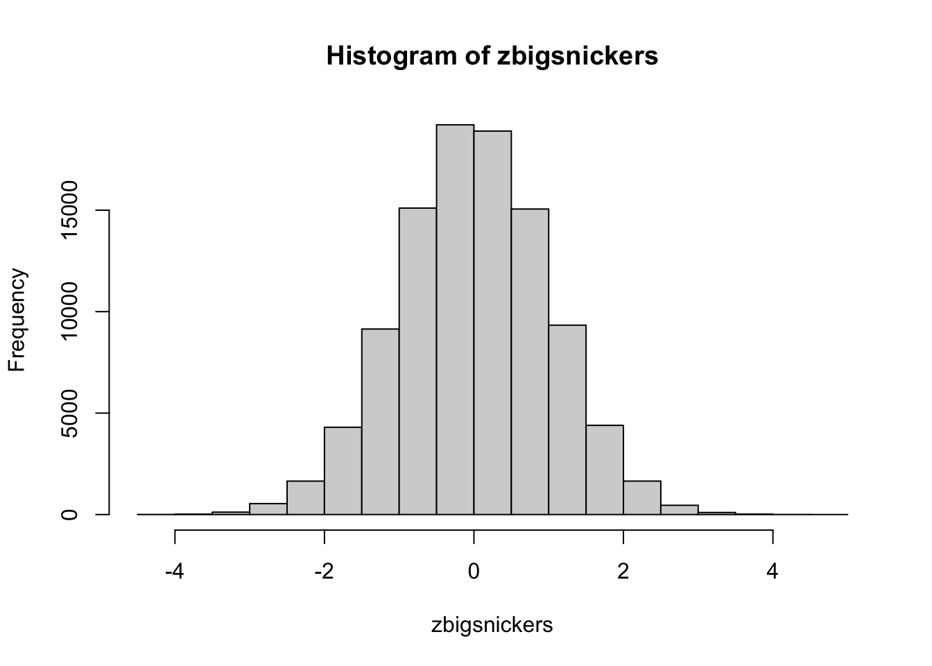
Figure 7.4: Histogram of Standardized Snickers Bar Weights (oz)
Here we see exactly what the process of standardizing values does for data that was already “bell shaped.” The distribution has the exact same shape, but the parameters of \(\mu\) and \(\sigma\) for the distribution have changed to 0 and 1.
Real data is rarely, if ever, perfectly Normal. However, what we are saying is that we can use a Normal random variable as a good predictive model for data like of that used in generating the bigsnickers dataset in Section 6.7.2.2.
As an analogy, it is likely not surprising to most people to learn that basic projectiles do not follow parabolic arcs, but we call can recall using a quadratic function to model the path of a cannonball, football, or some other basic projectile.
While the real world is rarely perfect, we can use some basic models to understand many phenomena. The Normal distribution is our primary model for continuous data and we will introduce the Binomial distribution as our primary model for discrete data in Chatper 8.
7.2 Finding the Probability from a Given Quantity.
The process of finding the probability associated to a given quantile is what we called the distribution function, \(\text{pdist}\), in Section 6.5. For Normal distributions, the distribution function is called pnorm() in R.
The syntax of pnorm() is
where the arguments are:
q: The bound (quantile) to be investigated.mean: The mean of the population being investigated. If no value is given,meanis set to0.sd: The standard deviation of the population being investigated. If no value is given,sdis set to1.lower.tail: This option controls whether the quantity returned is an upper or lower bound. Iflower.tail = TRUE(orT), then the output is the probability \(p\) such that \(P( x \leq q ) = p\). Iflower.tailis set toFALSE(orF), then the output is the probability \(p\) such that \(P(x > q) = p\). If no value is set, R will default tolower.tail = TRUE.
Example 7.2 (Eddie Gaedel) Eddie Gaedel85 has the distinction to be the shortest person to ever appear in a Major League Baseball game. Eddie stood 3 foot 7 inches (or 43 inches) tall when he appeared for the St. Louis Browns in 1951. If Eddie were alive today, he would be part of a population which has a mean of 69 inches and a population standard deviation of 3 inches.86
We can find the proportion of people who we expect to not be taller87 than Eddie using the following code.
## [1] 2.224776e-18The size of this number is not easy to comprehend. The number of males on Earth we expect to not be taller than Eddie can be found by multiplying the above probability by 4 billion.
## [1] 8.899104e-09Loosely speaking, this means that we would need to have a population over one hundred million times what is currently on Earth to statistically expect that an adult male of Eddie’s height would be on Earth.
The astute reader likely has realized that there are adult males alive who are shorter than Eddie was. However, if the population was truly Normal, we would not expect this to be the case. In fact, the National Health and Nutrition Examination Survey88 found that there was zero chance that a US male between the ages of 20 and 29 (Eddie was 26 at the time of his appearance with the Browns) below the height of 4 foot 11 inches and Eddie was a full 16 inches shorter than that.
Example 7.3 (Shaq and Britney) In Example 4.21, we used \(z\)-scores to answer the following question.
Shaquille O’Neal89, also known as Shaq, is a former professional basketball player and widely considered to be a cultural icon. Shaq stands at a staggering 7 foot 1 inch tall, or 85 inches tall. Britney Griner90 is a professional basketball player who has also entered the cultural discussion. Britney stands at 6 foot 9 inches tall, or 81 inches tall. If we ask the “kindergarten” question, “Who is taller?”, the answer is clear that Shaq is taller than Britney. However, a more nuanced question is whether Shaq is taller among men than Britney is among women.
We can now answer this question by finding the probability that a random male is taller than Shaq. Using the values of \(\mu_X = 69\) and \(\sigma_X = 3\) from both Examples 4.21 and 7.2 we get the following probability for Shaq.
## [1] 4.821303e-08This says that the probability that a random man is taller than Shaq is \({0.00000004821303}\).
For Britney, we will assume that US female heights are Normally distributed with \(\mu_X = 64.5\) and \(\sigma_X = 2.5\). We can find now the probability that a random US female is taller than Britney.
## [1] 2.055789e-11This says that the probability that a random woman is taller than Britney is \({0.00000000002055789}\).
While both of these probabilities are exceptionally small, we see that Britney gives rise to a much smaller value. In fact, if we were to calculate Britney’s percentile by setting lower.tail = TRUE, we get a surprising result.
## [1] 1This is saying that all people are no taller than Britney. This is technically incorrect as she is not the tallest woman in the world,91 but the p value here is so close to 1 that R simply returns 1.
According to the Law of Large Numbers (LLN), Theorem 6.1, we can say that there is virtually no difference between the probability of a random US adult male being taller than Shaq and the proportion of US adult males who are taller than Shaq.
That is, the LLN says there is no practical difference between proportions and probabilities.
7.3 Finding The Probabiltiy of Being Between Two Values
If we want to find the probability that a Normal random variable is between two values, we can use the Continuous Probability Axiom, Definition 6.7, that states
\[P(X = x_0) = 0\]
for any value \(x_0\) to get the following relations.
Theorem 7.2 If \(X\) is a continuous random variable, then the following are all equal.
\[P(a \leq X \leq b) = P(a < X \leq b) = P(a \leq X < b) = P(a < X < b)\] Moreover, we get that
\[P( X \leq a ) + P( a < X \leq b ) = P(X \leq b)\]
which gives that
\[P(a < X \leq b) = P(X\leq b) - P(X \leq a).\]
We can thus summarize how to use pnorm for this type of problem below.
If we are looking with a distribution with a population mean of mu and a population standard deviation of sigma, then we can find the value of \(P( a < X \leq b)\) with
Example 7.4 (Slightly Above Average Intelligence) IQ scores are standardized so that the values are Normally distributed with a mean of 100 and standard deviation of 15. To find the probability that a random person has an IQ between 100 and 115, we would use the code:
## [1] 0.3413447That is, the probability that a random person has an IQ between 100 and 115 is just a bit over 34%. We will revisit this setup in Section 7.5.
This exploration shows that if \(X\) is a Normal random variable modeling IQ scores, that \(P(124 < X \leq 148) \approx 0.0541\). It also shows that the \(P(X \leq 124) \approx 0.9452\) and that \(P(X>148)\approx 0.0007\).
Play around with the tool and answer the following questions.
What is the probability that a random person has an IQ less than 100? [Note: This one should be “obvious.”]
What is the probability that a random person has an IQ more than 120?
What is the probability that a random person has an IQ between 60 and 90?
7.4 Finding Quantities from Probabilities.
The quantile function \(\text{qdist}\) is used to find the quantity in a distribution that aligns with a certain probability. R has a built in function for Normal distributions called qnorm.
The syntax of qnorm() is
where the arguments are:
p: The probability to be bound by the output.mean: The mean of the population being investigated. If no value is given,meanis set to0.sd: The standard deviation of the population being investigated. If no value is given,sdis set to1.lower.tail: This option controls whether the quantity returned is an upper or lower bound. Iflower.tail = TRUE(orT), then the output is the quantity \(q\) such that \(P( x \leq q ) = p\). Iflower.tailis set toFALSE(orF), then the output is the quantity \(q\) such that \(P( x > q ) = p\). If no value is set, R will default tolower.tail = TRUE.
Example 7.5 (An IQ Example) To find the third quartile of IQ scores, we can use the following code.
## [1] 110.1173That is, we can say that three quarters or 75% of people have an IQ less than 111 (assuming values are rounded to the nearest integer).
Example 7.6 (Mensa) According to Mensa.org as of 10 September, 202492:
“Mensa is the world’s largest, oldest and most famous high IQ society.”
“In order to join Mensa, you have to take a Mensa-approved intelligence test that has been properly administered and supervised. And on that test you need to attain a score that places you within the upper 2% of the general population.”
If MENSA were to use an IQ score to determine eligibility, we can find the score that separates the top 2% of the population by running the code below.
## [1] 130.8062That is, a person should score at least 131 to ensure admission to Mensa.
Example 7.7 Say we wanted to find the middle 90% of IQ scores. This would mean that there would be 5% below and 5% above the range. To find these values we can use the following code:
## [1] 75.3272## [1] 124.6728which gives that the range is approximately between 75 and 125.
One could also find either of the above values, call it q, and then the other bound would be \(2\mu_{\scriptscriptstyle X} - q\).
7.5 The Empirical Rule
The Empirical Rule is a back-of-the-envelope calculation93 that gives estimates for a Normal distribution when \(z\) is among the values: \(-3, -2, -1, 0, 1, 2, 3\).
Theorem 7.3 The Empirical Rule states the following: \[\begin{align*} P( -1 < z \leq 1) & \approx 0.68\\ P( -2 < z \leq 2) & \approx 0.95\\ P( -3 < z \leq 3) & \approx 0.997 \end{align*}\]
Memorizing these values and recalling that any Normal distribution is symmetric allows a person to make approximations of areas such as \(P( -1 < z \leq2)\) with the use of some basic arithmetic.94
The exploration below can be used to find the probabilities/proportions associated to the Standard Normal Distribution.
Explore the Empirical Rule using the above tool and use it to answer the following questions.
Recall that IQ scores satisfy \(\text{Norm}(100,15)\).
Estimate the probability that a random person having an IQ between 100 and 115. (This is the problem that we investigated in Example 7.4.)
Estimate the probability that a random person has an IQ less than 70.
Estimate the probability that a random person has an IQ between 115 and 145.
Recall that the height of US adult males in inches can be approximated by \(\text{Norm}(69,3)\).
Estimate the probability that a random US adult male is over 6 feet tall.
Estimate the probability that a random US adult male is less than 5 foot 3 inches tall.
Estimate the probability that a random US adult male is between 5 foot 6 inches and 6 foot 3 inches tall.
Example 7.8 (Showing The Accuracy of The Empirical Rule) As we stated, the Empirical Rule just gives approximations. Using Theorem 7.2 and pnorm as discussed in Section 7.6 we get that
\[P( -n < z \leq n) = \text{pnorm( n )} - \text{pnorm( -n )}\] for any \(n>0\). We can now simply compare the calculated values from R with the approximated values from the Empirical Rule setting \(n\) to be 1, 2, and 3.
## [1] 0.6826895## [1] 0.9544997## [1] 0.9973002This shows that 68, 95, and 99.7% are reasonable approximations of the above values.
Example 7.9 (Foreshadowing Confidence Intervals) The Empirical Rule is also often used in reverse. One can say that approximately 95% of people have an IQ between \[\mu_{\scriptscriptstyle X} - 2 \sigma_{\scriptscriptstyle X} = 100 - 2 * 15 - 70\]
and
\[\mu_{\scriptscriptstyle X} + 2 \sigma_{\scriptscriptstyle X} = 100 + 2* 15 = 130.\]
To find the more precise bound for the middle \(68\% = 0.68\) we would first find the value of the probability in each tail. That is given by \(p = (1 - 0.68)/2 = 0.17\). That is, there is 17% in each of the left and right hand tails. The bounds are thus given by the following.
## [1] -0.9541653## [1] 0.9541653These are are more precise variations to the Empirical Rule’s approximated \(z = \pm 1\). The values for \(95\% = 0.95\) and \(99.7\% = 0.997\) are given below.
## [1] -1.959964## [1] 1.959964## [1] -2.967738## [1] 2.967738These are the more precise values of the Empirical Rule’s approximations of \(z = \pm 2\) and \(z = \pm 3\). In fact, we will see that \(z = \pm 1.96\) can be used as the critical value of \(z\) value when we do a 95% confidence interval using the Normal distribution as well as hypothesis testing based on \(z\) calculations.
In conclusion, the Empirical Rule is a very helpful tool for situations when data values occur either at precisely or nearly precisely the perfect \(z\)-values mentioned above. It is of worth note that the Empirical Rule will always under predict p values and that the quantiles that can be found from it are always just a bit too extreme.
7.6 p and q with \(z\).
Using the distribution and quantile functions are a major tool when working with a population that is Normal or can be closely modeled by a Normal distribution. It is important to be mindful of the similarities yet stark differences in the \(\text{pdist}\) and \(\text{qdist}\) functions for distributions that we discussed in Section 6.6. If one is working with or interested in standardized Normal values (or \(z\)-scores), then one can omit the mean and sd arguments of the Normal probability functions. For example, a 6 foot tall US male would have a \(z\)-score of 1, so the proportion of males who are not taller than 6 foot can be found with the following code.
## [1] 0.8413447or even simply
## [1] 0.8413447This is quickly checked with the Empirical Rule that says that the proportion of values between \(z = 0\) and \(z = 1\) is approximately 34% and the values with a negative \(z\)-score account for 50% of all observations. Therefore, the proportion of values with a \(z\)-score less than 1 is approximately 84% = 50% + 34%.
Conversely, if one wanted the \(z\)-score related to the top 2% of observations like we saw in Example 7.6 we would run the following.
## [1] 2.053749One can compare this to the value found earlier by using the formula \(\text{x} = \mu_{\scriptscriptstyle X} *\;\sigma_{\scriptscriptstyle X}\). This gives:
## [1] 130.8062which matches with what we found in Example 7.6.
7.7 The Random Normal Variable
This section is optional in a lot of introductory statistics courses.
Simulation is a powerful statistical and probabilistic tool and requires the generation of random values based on different distributions. To produce a random Normal value, we can use rnorm().
The syntax of rnorm() is
where the arguments are:
n: The number of random values that the user wants returned.mean: The mean of the population being investigated. If no value is given,meanis set to0.sd: The standard deviation of the population being investigated. If no value is given,sdis set to1.
Example 7.10 In Example 7.6 we saw that the \(z\)-score according to the top 2% of all values in a Normal distribution was 2.053749. So, if we ran rnorm a large number of times, we would only get an output larges than 2.053749 approximately 2% of the time.
This is quickly seen with the following calculation. [Here we use rnorm(0.98) instead of the version where lower.tail was set to FALSE that we were used in Example 7.6.] Refer to Chapter 13 for further discussions about using simulations.
## [1] 0.019977This shows that roughly 2% of randomly generated \(z\)-scores are greater than qnorm( 0.98 ). Running the code above again should offer another number approximately equal to 0.02 or 2%.
Review for Chapter 7
Chapter 7 Quiz: The Normal Distribution
This quiz tests your understanding of core concepts of the Normal Distribution, the Z-score, and the associated R functions presented in Chapter 7. The answers can be found prior to the Exercises section.
True or False: The \(z\)-score, or standardized value, tells you exactly how many standard deviations an individual observation is away from the mean of its distribution.
True or False: The Standard Normal Distribution is defined as the Normal distribution with a mean, \(\mu\), of 0 and a standard deviation, \(\sigma\), of 1.
True or False: The Empirical Rule (or 68-95-99.7 Rule) states that approximately 95% of the data in a Normal distribution falls within three standard deviations of the mean.
True or False: The Normal distribution is fundamentally a symmetric and unimodal distribution, where the mean, median, and mode are all equal.
True or False: The
pnorm()function calculates the probability that a variable is no more than a given \(x\)-value or \(z\)-score.True or False: By default, the
pnorm()function calculates the area in the upper tail (area greater than the value) unless the argumentlower.tail = TRUEis used.True or False: A negative Z-score indicates that the observed value is less than the distribution’s mean.
True or False: The primary purpose of converting an observation to a Z-score is to allow for the comparison of values taken from two different Normal distributions.
True or False: The Quantile R function,
qnorm(), is used to find a value of \(x\) (or \(z\)) that corresponds to a specified percentile (area).True or False: The Central Limit Theorem (CLT) is important to the Normal Distribution because it allows the tools of the Normal Distribution to be used to analyze samples taken from many other, non-Normal distributions.
Definitions
Section 7.1
Definition 7.1 \(\;\) A population that gives the density function below is said to be the Normal Distribution with Mean of \(\mu\) and Standard Deviation of \(\sigma\), denoted \({\bf \text{Norm}(\mu, \sigma)}\) for short.
\[\text{ddist}(x) = \frac{1}{\sigma \sqrt{2\pi}}e^{\frac{-1}{2}\left( \frac {x-\mu}{\sigma} \right)^2}\] In particular, we will refer to \(\text{Norm}(0,1)\) as the Standard Normal Distribution. A graph of the Standard Normal distribution is shown below.
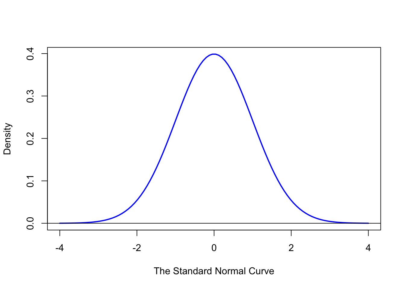
Figure 7.5: Standard Normal Density Function
Results
Section 7.1
Section 7.3
Theorem 7.2 \(\;\) If \(X\) is a continuous random variable, then the following are all equal.
\[P(a \leq X \leq b) = P(a < X \leq b) = P(a \leq X < b) = P(a < X < b)\] Moreover, we get that
\[P( X \leq a ) + P( a < X \leq b ) = P(X \leq b)\]
which gives that
\[P(a < X \leq b) = P(X\leq b) - P(X \leq a).\]
Big Ideas
Section 7.1
Real data is rarely, if ever, perfectly Normal. However, what we are saying is that we can use a Normal random variable as a good predictive model for data like of that used in generating the bigsnickers dataset in Section 6.7.2.2.
As an analogy, it is likely not surprising to most people to learn that basic projectiles do not follow parabolic arcs, but we call can recall using a quadratic function to model the path of a cannonball, football, or some other basic projectile.
While the real world is rarely perfect, we can use some basic models to understand many phenomena. The Normal distribution is our primary model for continuous data and we will introduce the Binomial distribution as our primary model for discrete data in Chatper 8.
Section 7.2
According to the Law of Large Numbers (LLN), Theorem 6.1, we can say that there is virtually no difference between the probability of a random US adult male being taller than Shaq and the proportion of US adult males who are taller than Shaq.
That is, the LLN says there is no practical difference between proportions and probabilities.
Important Remarks
Section 7.1
We will NOT use the formula in Definition 7.1 for anything other than to give an explicit definition of the Normal distributions. It can be found in R as
dnorm, however.It is assumed in Definition 7.1 that \(\sigma > 0\).
We will always capitalize the word Normal when in the context of a Normal distribution. Thus, if we say a distribution is Normal, we mean that it satisfies Definition 7.1.
We have defined the population mean and standard deviation of a Normal distribution, but these definitions agree with all other valid definitions for such a distribution. We will explore a geometric interpretation of these values shortly.
For a more rigorous take on the population parameters \(\mu\) and \(\sigma\) of the Normal random variable, see Chapter 4 of Probability, Statistics, and Data: A Fresh Approach Using R.
Code Templates
Section 7.3
New Functions
Section 7.2
The syntax of pnorm() is
where the arguments are:
q: The bound (quantile) to be investigated.mean: The mean of the population being investigated. If no value is given,meanis set to0.sd: The standard deviation of the population being investigated. If no value is given,sdis set to1.lower.tail: This option controls whether the quantity returned is an upper or lower bound. Iflower.tail = TRUE(orT), then the output is the probability \(p\) such that \(P( x \leq q ) = p\). Iflower.tailis set toFALSE(orF), then the output is the probability \(p\) such that \(P(x > q) = p\). If no value is set, R will default tolower.tail = TRUE.
Section 7.4
The syntax of qnorm() is
where the arguments are:
p: The probability to be bound by the output.mean: The mean of the population being investigated. If no value is given,meanis set to0.sd: The standard deviation of the population being investigated. If no value is given,sdis set to1.lower.tail: This option controls whether the quantity returned is an upper or lower bound. Iflower.tail = TRUE(orT), then the output is the quantity \(q\) such that \(P( x \leq q ) = p\). Iflower.tailis set toFALSE(orF), then the output is the quantity \(q\) such that \(P( x > q ) = p\). If no value is set, R will default tolower.tail = TRUE.
Section 7.7
The syntax of rnorm() is
where the arguments are:
n: The number of random values that the user wants returned.mean: The mean of the population being investigated. If no value is given,meanis set to0.sd: The standard deviation of the population being investigated. If no value is given,sdis set to1.
Exercises
Exercise 7.1 What IQ score is needed to be in the top 1% of the population?
Exercise 7.2 Robert Wadlow95 had the distinction of being the tallest person in recorded history. Assuming we use the same \(\mu_{\scriptscriptstyle X}\) and \(\sigma_{\scriptscriptstyle X}\) that we used for Shaq in Example 7.3, what is the probability that a random US male is taller than the Robert was at his death, 8 foot 11.1 inches? To offer some context, take the reciprocal of this value to say that the probability is 1 out of how many people? [Hint: As an example, if the probability was 0.25, then 1/0.25 = 4 and we could say that the probability is 1 in 4.]
Exercise 7.3 How tall would a US woman have to be to be as tall as Robert Wadlow was among men? Assume the values for \(\mu_{\scriptscriptstyle X}\) and \(\sigma_{\scriptscriptstyle X}\) for both men and women are the same as used in Example 7.3.
Exercise 7.4 How high of an IQ score would a person have to be to be as “smart” as Shaq is tall?
Exercise 7.5 What is the probability that a random person has an IQ higher than Albert Einstein had? [It is purported that Einstein’s IQ was approximately 160.]
Exercise 7.6 Find the first quartile for IQ scores.
Exercise 7.7 Find the third quartile for the distribution of the birth weights of baby girls and give a practical interpretation of this quantity. [You may assume that the population is Normally distributed with \(\mu_X\) being 7 pounds 5 ounces and \(\sigma_X\) being 1 pound 2 ounces.]
Fauna of Australia. Vol. 1b. Australian Biological Resources Study (ABRS)↩︎
In fact, if we found the average of 15 dice, then a sample of 1000 trials will likely “pass” the QQ analysis that we derive later in Section 14.1 to test the underlying population for Normality.↩︎
Eddie appeared for the St. Louis Browns in the second game of a doubleheader on 19 August, 1951. See Wikipedia for more information.↩︎
The exact values of the mean and standard deviation are not widely agreed upon. We have used values here which are not vastly different than any of the values that the author could find.↩︎
This will be an unfortunate theme of somewhat awkward language in order to be completely precise. Because the
lower.tail = TRUEoption gives the probability \(P( x \leq q )\) we cannot say the proportion of people who are shorter than Eddie. This is just one example when we must use complicated language to represent expressions relating to the inequalities “\(\leq\)” and “\(\geq\)”.↩︎See https://www2.census.gov/library/publications/2010/compendia/statab/130ed/tables/11s0205.pdf↩︎
According to Wikipedia, Rumeysa Gelgi is the tallest living woman at the time of publication. She was measured at 7 foot and 0.71 inches in May 2021.↩︎
A “back-of-the-envelope calculation” is a calculation which can be made quickly without any fancy computational equipment to give a good approximation to a value in question. See Wikipedia for more.↩︎
The Empirical Rule would approximate this value at 81.5% while R would give a value of 0.8185946.↩︎
The life and growth of Robert Wadlow is hard to comprehend even when one is confronted with the literal facts. The curious reader is encouraged to see Wikipedia for more information.↩︎