Chapter 4 Numerical Summaries of Data
Figure 4.1: A Statypus Begins Working on Some Advanced Theoretical Statistics
A baby platypus has a name that is as cute as it is. A baby platypus is called a puggle.49
Data sets can have thousands, millions, or even billions of values. It is often beneficial to have numeric values which summarize these data. The concept of “average” is handled in statistics with values such as the arithmetic mean, which we will often just call the mean, and median. There are other values which play into the concept of “average,” but we will focus on these two for now. While these measures give a summary of the center of a data set, how varied the set is is also of importance. There would not be a need for any investigation if data values did not vary and it is a cornerstone of statistical thinking to understand how data values differ within a sample or population. We will measure the level of variability or dispersion using the values of standard deviation and interquartile range. These tools offer us a language to discuss the shape of a data set which we can also see using a box plot.
New R Functions Used
All functions listed below have a help file built into RStudio. Most of these functions have options which are not fully covered or not mentioned in this chapter. To access more information about other functionality and uses for these functions, use the ? command. E.g. To see the help file for summary, you can run ?summary or ?summary() in either an R Script or in your Console.
We will see the following functions in Chapter 4.
mean(): A generic function for the (trimmed) arithmetic mean.median(): Computes the sample median.min(): Returns the minimum of the input values.max(): Returns the maximum of the input values.range(): Returns a vector containing the minimum and maximum of all the given arguments.summary(): A generic function used to produce result summaries of the data.IQR(): Computes interquartile range of thexvalues.sd(): Computes the standard deviation of the values inx.boxplot(): Produces box-and-whisker plot(s) of the given values.quantile(): Produces sample quantiles corresponding to the given probabilities.
There are additional functions given in the appendix which can be of benefit if the built-in R functions do not agree with an automated homework system. These functions were developed at Saint Louis University. Please contact Dr. Phil Huling at phil.huling@slu.edu if you have further questions about their functionality.
To load all of the datasets used in Chapter 4, run the following line of code.
4.1 Measures of Central Tendency
The term “average” is often used in everyday language to discuss something that somehow represents a typical value of a set. In modern statistics, the two most basic examples of this type of value for numerical data are the median and mean, or arithmetic mean to be more precise.
While some statistics courses also discuss the mode in conjunction with the median and mean, it is not a measure of central tendency. In fact, it is quite possible for the mode to be either the minimum or maximum value of a dataset.
Both the mean and the median are meant to measure the center of a set of data in some sense. They do so in different ways and in this section, we will try to give some insight on what each is doing.
We first consider the arithmetic mean. Pretend we had a set of \(n\) values, \(\left\{ x_1, x_2, \ldots, x_n \right\}\) and wanted to find a single value, call it \(m\), that somehow represents all of them simultaneously. In all but the silliest of cases, most of our values will not equal \(m\) but have some deviation from it. We can find these deviations by summing up the values of \(x_i - m\) and calling the sum \(E\).
\[\begin{align*} E &= (x_1-m)+ (x_2-m)+ \cdots + (x_n-m) \\ &= (x_1 + x_2 + \cdots + x_n) - \underbrace{( m + m + \cdots + m)}_{n \text{ copies}} \\ &= (x_1 + x_2 + \cdots + x_n) - n\cdot m \end{align*}\]
Since \(E\) is literally the sum of all the “errors” that \(m\) would give, it makes sense to want \(E = 0\). We can force this by setting \(E=0\) and solving for \(m\).
\[ m = \frac{x_1 + x_2 + \cdots + x_n}{n}\]
This tells us that the arithmetic mean, or simply mean, is the unique value that makes the sum of the deviations equal to 0.
Another way of thinking about this is to consider this is as follows. First we break the \(x_i\) values into three groups: the values larger than the mean, those equal to the mean, and those smaller than the mean. Then we consider the deviations from each group. The deviations from the first group would be positive. The deviations from the second group would all be zero. Finally, the deviations from the final group would all be negative. Since the sum of all the deviations is forced to be zero, we get that the sum of the positive deviations is the opposite of the sum of the negative deviations. This is equivalent to saying that the sum of the lengths of the positive deviations is equal to the lengths of the negative deviations. This is one way to find the center of the values.
We can visualize this with an exploration.
We can change the value of any of the values by dragging the highlighted blue dots. If you toggle the switch labeled “Show Mean” to read “Yes,” you can display a dotted gray line that shows the arithmetic mean of the values. Toggle this switch to select “Yes.”
The purple line is a value we can manipulate by dragging the dot on the vertical axis. Initially, the purple line should be aligned with the dotted gray line and the green toggle switch should be set to “Mean.”
The value under “Sum of blue” represents the sum of all the positive deviations from the purple line and the value under “Sum of red” represents the sum of all the lengths of the negative deviations from the purple line. Initially, because the purple line is aligned with the gray one, the values of “Sum of blue” and “Sum of red” are equal. However, if you move the purple dot up and down, you will see that the only place that makes the red and blue lengths equal is at the gray line.
If you drag any of the highlighted blue dots, the gray line will move dynamically to match the mean of the values. Whatever we set the values to be, we quickly see that the only way to make “Sum of blue” to be equal to “Sum of red” is to make the purple line exactly aligned with the gray line.
You can also add a fifth variable value by toggling the switch labeled “Points” to read “Odd.”
There is another, and in some ways, simpler way of trying to find the “center” of a dataset. A value that has the property that half of the values in a dataset are less than it and half of the values are greater than it is what we want to call the median. We will return to the above exploration to see how this plays out.
We will once again use the exploration above which can be found below.
We begin by toggling the green “switch” from Mean to Median. This should change the red and blue outputs on the left side of the exploration as well. It should now show the number of values above the purple line in blue and the number of values below the purple line in red. Initially, we should see that there is only one value above the purple line and three values below it. We can drag the purple slider on the vertical axis down to equalize this and quickly find that any value between 2 and 3 (exclusive) makes both the blue and red values both be 2. In a certain sense we could take any value in this range to be the median, but will see in Section 4.1.2 that we will set a method for determining it precisely for a given dataset.
4.1.1 Mean
We can formalize our exploration of the mean as follows. The arithmetic mean or just simply mean is a measure of central tendency that gives the “average” value if we are looking at adding up the values. Equivalent to our derivation above, if there are \(n\) values in a vector, \({\bf x}\), then the mean, or \(\bar{x}\), is a value such that adding \(n\) copies of the mean, \(\bar{x}\), would equal the sum of the values in \({\bf x}\). That is, we have
\[x_1+x_2+\cdots+x_n = \sum_{i = 1}^n x_i = \sum_{i = 1}^n \bar{x} = \underbrace{\bar{x} + \bar{x} + \cdots + \bar{x}}_{n \text{ copies}} = n \cdot \bar{x}\] We are now set to formally define both the mean and deviations of a set of data.
Definition 4.1 Given a vector \({\bf x} = ( x_1, x_2, \ldots, x_n )\) having \(n\) values, we can define the arithmetic mean or simply mean of \({\bf x}\), which we denote as \(\bar{x}\) if \({\bf x}\) is a sample or \(\mu\) if \({\bf x}\) is the entire population, as follows. \[\bar{x} \text{ or }\mu= \frac{1}{n} \sum_{i = 1}^n x_i = \frac{1}{n} \left( x_1 + x_2 + \cdots + x_n \right) = \frac{ x_1 + x_2 + \cdots + x_n }{n}.\]
It is important to make a distinction between a population mean, denoted as \(\mu\), which is a parameter and a sample mean, denoted \(\bar{x}\), which is a statistic. Often, we are unable to work with an entire population, so we will often be using a sample to calculate \(\bar{x}\) which will be our best guess for \(\mu\). As mentioned in Chapter 2, this will be a common thread throughout our work. We will often default to denoting a mean as \(\bar{x}\) when working with data as often we will only be able to work with a sample of a population.
Now that we have the defined the mean, we can give a definition to the concept of a deviation which we used in Section 4.1.
Definition 4.2 The Deviation of a Value, \(x_i\), of a vector \({{\bf x} = ( x_1, x_2, \ldots, x_n)}\), is defined as \[ \text{dev}(x_i) = x_i - \bar{x}\] or \[ \text{dev}(x_i) = x_i - \mu.\] We define the Deviation of a Vector to be the vector of its deviations. That is,
\[\text{dev}({\bf x}) = \left(\text{dev}(x_1), \text{dev}(x_2), \ldots, \text{dev}(x_n) \right).\]
We will return to this concept in Section 4.2.4
We can manually calculate the mean of a vector x with the following code.
As an example, let x be the vector of the integers from 2 to 11 which we can set with the following line of code.
## [1] 2 3 4 5 6 7 8 9 10 11and then find \(\bar{x}\) via the above where we now append the line of xbar to output the result.
## [1] 6.5Of course, R has a built in function for this as well, mean().
The syntax of mean is
where the argument is
na.rm: A logical ofTRUEorFALSEindicating whetherNAvalues should be stripped before the computation proceeds.
The function mean() can be utilized on a vector, x, via
or on the column named ColName of a dataframe named df via
As a quick example, we can revisit x <- 2:11 using mean().
## [1] 6.5We see that this matches our manual calculation.
Example 4.1 We will begin by importing a data frame which contains variables about a sample of 200 births during the year of 1998 as recorded by the U.S.Department of Health and Human Services.
Use the following code to download BabyData1.
It is recommended that you run the str and head functions whenever you import a new dataset.
## 'data.frame':    200 obs. of  12 variables:
##  $ mom_age      : int  35 22 35 23 23 26 25 32 41 22 ...
##  $ dad_age      : int  35 21 42 NA 28 31 37 38 39 24 ...
##  $ mom_educ     : int  6 3 4 1 4 3 5 5 4 3 ...
##  $ mom_marital  : int  1 1 1 1 1 2 1 1 1 2 ...
##  $ numlive      : int  2 1 0 2 0 1 0 1 0 0 ...
##  $ dobmm        : int  2 3 6 8 9 10 7 12 11 2 ...
##  $ gestation    : int  39 42 39 40 42 39 38 38 36 40 ...
##  $ sex          : chr  "F" "F" "F" "F" ...
##  $ weight       : int  3175 3884 3030 3629 3481 3374 2693 4338 2834 2948 ...
##  $ prenatalstart: int  1 2 2 1 2 4 1 1 2 1 ...
##  $ orig_id      : int  1047483 1468100 2260016 3583052 795674 3544316 3726920 2606970 2481971 243759 ...
## $ preemie : logi FALSE FALSE FALSE FALSE FALSE FALSE ...## mom_age dad_age mom_educ mom_marital numlive dobmm gestation sex weight
## 1 35 35 6 1 2 2 39 F 3175
## 2 22 21 3 1 1 3 42 F 3884
## 3 35 42 4 1 0 6 39 F 3030
## 4 23 NA 1 1 2 8 40 F 3629
## 5 23 28 4 1 0 9 42 F 3481
## 6 26 31 3 2 1 10 39 M 3374
## prenatalstart orig_id preemie
## 1 1 1047483 FALSE
## 2 2 1468100 FALSE
## 3 2 2260016 FALSE
## 4 1 3583052 FALSE
## 5 2 795674 FALSE
## 6 4 3544316 FALSEYou can also use the View function to place the data frame into the viewing window which is, typically, in the upper left pane of RStudio.
We can find the mean age of the mother of the babies with the following code.
## [1] 26.585A common error functions can run into is trying to evaluate a numerical summary when a vector, or column of a data frame, has either missing values or entries such as “NA”. If you look at the data in BabyData1$dad_age, you will notice that not all of the values exist. As such, when R tries to find the median, it runs into an issue and returns the following.
## [1] NAIf you run a numerical function and obtain NA as the output, this can often be easily fixed by simply amending the option na.rm = TRUE inside the function as shown below.
## [1] 30.06024It is not really an error that mean returns NA when the dataset contains a missing value, but instead it should be viewed as R letting you know of the missing value and requiring you to acknowledge those missing value before it will remove them to make the calculation.
4.1.2 Median
We could define a Median as a specific number such that at least half of the values in a dataset are at least that number and at least half of the values are at most that number. However, as we saw in our exploration earlier, this would not lead to a unique definition of the median. We can now give a definition which will unambiguously define the median for any finite sized dataset.
Definition 4.3 Let \({\bf x}\) be a vector of \(n\) values, \((x_1, x_2, \ldots, x_n)\). We can reorder them and (possibly) relabel them as \((w_1, w_2, \ldots, w_n)\) such that \(w_1 \leq w_2 \leq \cdots \leq w_n\) and each \(w_i\) is some \(x_j.\) We can define the Median of \({\bf x}\) based on the parity of \(n\), i.e. whether it is even or odd.
If \(n\) is odd, then let \(L = \frac{n-1}{2}\) (which means \(n = 2L + 1\)) and we define the Median of \(x\) to be \(w_{L+1}\).
If \(n\) is even, then let \(K = \frac{n}{2}\) (which means that \(n = 2K\)) and we define the Median of \({\bf x}\) to be the value \(\frac{w_K + w_{K+1}}{2}\), or the arithmetic mean of the two most “middle” values of \({\bf x}\).
Example 4.2 To do this manually, we will work with mtcars$mpg.
##  [1] 21.0 21.0 22.8 21.4 18.7 18.1 14.3 24.4 22.8 19.2 17.8 16.4 17.3 15.2 10.4
## [16] 10.4 14.7 32.4 30.4 33.9 21.5 15.5 15.2 13.3 19.2 27.3 26.0 30.4 15.8 19.7
## [31] 15.0 21.4
These values are not in order, so we begin by sorting the dataset using the sort function we first saw in Section 2.5.1.2.
##  [1] 10.4 10.4 13.3 14.3 14.7 15.0 15.2 15.2 15.5 15.8 16.4 17.3 17.8 18.1 18.7
## [16] 19.2 19.2 19.7 21.0 21.0 21.4 21.4 21.5 22.8 22.8 24.4 26.0 27.3 30.4 30.4
## [31] 32.4 33.9
Here we have that mtcars$mpg is \({\bf x}\) and carssorted is \((w_1, w_2, \ldots, w_n)\). We can now find the length of either mtcars$mpg or carssorted and store it as n.
## [1] 32Since \(n\) is even, we calculate \(K= \frac{n}{2}\) and find the mean of the \(K\)th and \((K+1)\)th value of carssorted.
## [1] 19.2Thus, the median of mtcars$mpg is 11.85 which means that half of the cars had a fuel efficiency less than 11.85 mpg and half of cars had a fuel efficiency more than 11.85 mpg.
There is, obviously, a built in function for this in R, median().
The syntax of median is
where the argument is
na.rm: A logical ofTRUEorFALSEindicating whetherNAvalues should be stripped before the computation proceeds.
We can check that this agrees with our manual calculations for mtcars$mpg:
## [1] 19.2The function median can be utilized on a vector, x, via
or on the column named ColName of a dataframe named df via
Example 4.3 We can revisit the BabyData1 dataframe which we first saw (and imported) in Example 4.1. We can find the median age of the birth mother using the following code.
## [1] 26Unfortunately, like mean, median will also not return a value if the vector is missing any values.
## [1] NAFortunately, the fix is the same as before.
## [1] 29.5We will return to the differences between the mean and median in Section 4.5 where we investigate how much extreme values affect these values.
4.2 Measures of Variability
Consider the two vectors below:
Both of the vectors have both the mean and median equaling 3 (which you are encouraged to verify in R), while it is clear that the vectors are different. The center of the data sets may be the same, but yVec has no variability while xVec has all unique values.
We will now introduce different measures, which we will call Measures of Variability, to be able to distinguish datasets based on how varied the values are.
4.2.1 Range
The simplest way to discuss the variability of a dataset is what we call the Range.
Definition 4.4 Given a finite list of quantitative values, \(x\), we define the Range of \(x\) to be the interval \([ \text{min}, \text{Max}]\) where \(\text{min}\) is the minimum value of \(x\) and \(\text{Max}\) is the maximum value.
R has built in functions to find the minimum and maximum values, which are min() and max() respectively.50
The syntax of min is
where the argument is
na.rm: A logical ofTRUEorFALSEindicating whetherNAvalues should be stripped before the computation proceeds.
The syntax of max is
where the argument is
na.rm: A logical ofTRUEorFALSEindicating whetherNAvalues should be stripped before the computation proceeds.
The R software can find the range interval directly using the base R function called, not surprisingly, range().
The syntax of range is
where the argument is
na.rm: A logical ofTRUEorFALSEindicating whetherNAvalues should be stripped before the computation proceeds.
Running the following code shows that range returns a vector containing the minimum and maximum of all the given arguments.
## [1] 1 5## [1] 3 3This says that the values of xVec are in between 1 and 5 inclusively and the values of yVec are between 3 and 3 inclusively (and thus all the values must be 3).
The line of code to find the range of xVec may be better written as below.
Here we explicitly label the argument we are giving the range function. This is indeed best practice when using most functions, but we may omit the explicit argument names on functions when we are only providing a single argument.
The range function can be utilized on a vector, x, via
or on the column named ColName of a dataframe named df via
Some books define the range of a vector to be the difference of the maximum and minimum and not the ordered pair/interval. We will use the following definition when necessary.
Definition 4.5 If a dataset has a range of \([\text{min}, \text{Max}]\), then the Range Length is defined to be the value \(\text{Max}-\text{min}\).
Example 4.4 If we wanted to find the range of birth masses of babies in our sample, we can do this with the following code.
## [1] 907 4825This shows us that the smallest baby in our sample had a mass 907 grams while the largest had a mass of 4825 grams.
The range length is thus \(4825 - 907 = 3918\) grams.
4.2.2 Quartiles
While the median found the center of an ordered list of values, the quartiles attempt to find the medians of the lower and upper half of the now split vector. We want to define the Quartiles of a dataset to be a collection of five numbers, denoted \(Q_0, Q_1, Q_2, Q_3, \text{ and } Q_4\). We will insist that \(Q_0\) is the minimum value of the dataset, \(Q_2\) is the median of the dataset, and \(Q_4\) is the maximum value of the dataset. That is, it is the following set of numbers which are often collectively called the Five Number Summary.
\[ Q_0 = \text{Min.}\leq Q_1 \leq Q_2 = \text{Median} \leq Q_3 \leq Q_4 = \text{Max}.\]
Definition 4.6 For \(k =0,1,2,3,4\), the \(k\)th Quartile, \(Q_k\) is a number such that at least the proportion \(\frac{k}{4}\) of the values in the dataset are no more than \(Q_k\) and at least the proportion \(1-\frac{k}{4}\) of the values are no less than \(Q_k\). We also require that \(Q_2\) is the median of the dataset (as defined in Definition 4.3) and that \(Q_0\) and \(Q_4\) are \(\text{min}\) and \(\text{Max}\) (as defined in Definition 4.4) respectively.
This agrees with our conventions for \(Q_0\), \(Q_2\), and \(Q_4\) by definition, but leaves ambiguity for \(Q_1\) and \(Q_3\). The five number summary, specifically \(Q_1\) and \(Q_3\), can be calculated in many different ways.
In this book, we will adopt the convention to call any group of numbers, \(Q_k\) for \(k = 0,1,2,3,4\), that satisfies Definition 4.6 a “Five Number Summary.”
Leaving the ambiguity in the definition suggests that there are various valid ways of defining \(Q_1\) and \(Q_3\). While we will allow any acceptable set of five numbers to be a five number summary, we will default to using the summary() function to find a five number summary for our dataset.
The summary() functions returns the five quartiles as well as the mean (positioned between the median and third quartile). It can also be used on a data frame. Along with head and str, it is a good function to run on any new quantitative dataset you encounter to get a quick look at its characteristics.
The syntax of summary is
where the argument is
object: An object for which a summary is desired.
There are other options/arguments we could use with summary, but we will focus on using it for a quick look at the data, a way to find the quartiles of a dataset, and see how the mean compares to the median.
This summary function can be utilized on a vector, x, via
or on the column named ColName of a dataframe named df via
If you run
on a data frame, df, it will return the result of summary for each column. The results for non-quantitative variables may yield varied results.
Example 4.5 Using the BabyData1 dataframe again, we can get the quartiles (as well as the mean) for BabyData1$mom_age by running the following line of code.
##    Min. 1st Qu.  Median    Mean 3rd Qu.    Max.
##   14.00   21.00   26.00   26.59   31.25   42.00
This returns the five number summary of the age of the mothers as well as the mean.
We can also run summary on the entire BabyData1 dataframe to see what summary does for different kinds of data.
##     mom_age         dad_age         mom_educ      mom_marital       numlive
##  Min.   :14.00   Min.   :18.00   Min.   :1.000   Min.   :1.000   Min.   :0.00
##  1st Qu.:21.00   1st Qu.:24.00   1st Qu.:3.000   1st Qu.:1.000   1st Qu.:0.00
##  Median :26.00   Median :29.50   Median :3.000   Median :1.000   Median :1.00
##  Mean   :26.59   Mean   :30.06   Mean   :3.489   Mean   :1.385   Mean   :0.92
##  3rd Qu.:31.25   3rd Qu.:35.00   3rd Qu.:4.000   3rd Qu.:2.000   3rd Qu.:1.00
##  Max.   :42.00   Max.   :48.00   Max.   :6.000   Max.   :2.000   Max.   :5.00
##                  NAs    :34      NAs    :12
##      dobmm         gestation            sex          weight     prenatalstart
##  Min.   : 1.00   Min.   :23.00   Length   :200   Min.   : 907   Min.   :0.0
##  1st Qu.: 3.00   1st Qu.:38.00   N.unique :  2   1st Qu.:2935   1st Qu.:2.0
##  Median : 7.00   Median :39.00   N.blank  :  0   Median :3325   Median :2.0
##  Mean   : 6.54   Mean   :38.92   Min.nchar:  1   Mean   :3283   Mean   :2.4
##  3rd Qu.: 9.25   3rd Qu.:40.00   Max.nchar:  1   3rd Qu.:3629   3rd Qu.:3.0
##  Max.   :12.00   Max.   :47.00                   Max.   :4825   Max.   :9.0
##                                                                 NAs    :5
##     orig_id         preemie
##  Min.   :  51593   Mode :logical
##  1st Qu.:1158653   FALSE:174
##  Median :1994176   TRUE :26
##  Mean   :2042214
##  3rd Qu.:2929115
##  Max.   :3916227
##
Unlike other functions, summary will still return meaningful information even if the data set has any NA entries. In fact, summary adds an additional column which counts the number of NA entries in the vector.
We can see this with looking at the information about dad_age above. We also see the result of running summary on a chr type variable for the sex variable as well as how summary handles logical values for preemie.
Unfortunately, a lot of introductory statistics textbooks define the quartiles in a way that is inconsistent with R functions. If you need R output to match an online homework system, there are functions in this chapter’s appendix, Section 4.6, which give output which match a lot of introductory statistic textbooks.
Even R has alternative ways to calculate quartiles. We will see one method when we get to the quantile() function. You can also try the function fivenum() on a numeric vector, e.g. BabyData1$dad_age.
4.2.3 Interquartile Range
While the range is a measure of variability, it is determined only by the most extreme values of a dataset. A better measure of variability that uses the quartiles is what we call the Interquartile Range.
Definition 4.7 The Interquartile Range of a dataset is defined to be the interval \([Q_1, Q_3]\). We also define the Interquartile Range Length to be the value \(Q_3 - Q_1\).
- A lot of books define the interquartile range to be what we have called the interquartile range length. We have chosen this notation to make it consistent with that of range.
- We may blur between the interquartile range and the interquartile range length and hope that context will make the situation clear.
- Due to our lack of uniqueness in defining \(Q_1\) and \(Q_3\), there is some ambiguity in our definition of both the interquartile range and the interquartile range length. In practice, simply supplying the code used to make a calculation will remove this issue.
The interquartile range length, or simply IQR, can be found in RStudio by subtracting the first quartile from the third quartile using summary or directly with the IQR() function.
The syntax of IQR is
where the argument is
na.rm: A logical ofTRUEorFALSEindicating whetherNAvalues should be stripped before the computation proceeds.
In most cases, we can simply run IQR as follows.
#Will only run if x is defined
IQR( x )
#Will only run if df is appropriately defined
IQR( df$ColName )
Where the user has the option to include the argument na.rm = TRUE if they want to omit NA values.
Quartile calculations can be done in many ways and using summary() and IQR() will not always agree. There are functions in the appendix of this chapter that will give versions which will agree with a lot of other introductory statistics textbooks.
Example 4.6 state.area is a data vector built into RStudio which gives the area of the fifty US states in alphabetical order of the state name. We can find the IQR of state.area by either running
##    Min. 1st Qu.  Median    Mean 3rd Qu.    Max.
##    1214   37317   56222   72368   83234  589757
and then calculating
## [1] 45917or simply by using
## [1] 45916.75This is an example of where the different calculation methods for IQR can give very similar, but not identical results.
4.2.4 Sample Standard Deviation
While the IQR is a good measure of variability that works well with the median, the standard deviation is the measure that more naturally plays with the mean. It accounts for how far from each value is from the mean and attempts to minimize the deviation from the mean.
Definition 4.8 Given a vector \({\bf x} = ( x_1, x_2, \ldots, x_n )\) having \(n\) values (with \(n\geq 2\)), we can define the Sample Standard Deviation of \({\bf x}\), denoted by \(s_{\bf x}\) (or simply \(s\) when there is a low chance of confusion), to be
\[ s_{\bf x} = \sqrt{ \frac{\displaystyle{\sum \left( x_i - \bar{x}\right)^2}}{n-1}}.\] We can also define the Sample Variance to be the square of the sample standard deviation. That is, the sample variance is \[ s_{\bf x}^2 = \frac{\displaystyle{\sum \left( x_i - \bar{x}\right)^2}}{n-1}.\] In both cases, we say that the value \(n-1\) is the Degrees of Freedom and will later denote it by the Greek letter \(\nu\), pronounced like “new.”
The Standard Deviation is a measure of spread that provides an estimate of the average distance of each observation from the mean.
The standard deviation is never negative and 0 exactly when all the values of a dataset are identical.
It is logically equivalent to think of the sample standard deviation as being the square root of the variance or the sample variance as being the square of the sample standard deviation. For most of this book, the sample standard deviation will be a more “fundamental” tool for us, so we will adopt the idea of viewing the variance as the square of the standard deviation.
Example 4.7 We will work through the definition of the sample standard deviation with our “toy” vector of x <- 2:11 from before. We first begin by finding the mean of x (again).
To see how good of an estimator \(\bar{x}\) is of x, we can calculate the deviations of x, \(x - \bar{x}\). We save the deviations as Devx.
## [1] -4.5 -3.5 -2.5 -1.5 -0.5 0.5 1.5 2.5 3.5 4.5We note that the deviations sum to 0 which we used to derive the formula for \(\bar{x}\) in Section 4.1.
## [1] 0This means that if we know \(n-1\) of the deviations, we, in fact, know all of them because the remaining deviation is necessarily the opposite of the sum of the other \(n-1\) deviations. This is precisely why we will choose to divide by \(n-1\) shortly rather than \(n\) and say that a sample of size \(n\) has \(n-1\) degrees of freedom.
To avoid the cancellation of the deviations, we calculate the sum of the squares of Devx, which we cleverly call SumSquareDevx.
## [1] 82.5We have thus far found
\[\sum_{i=1}^n \left(x_i - \bar{x}\right)^2.\]
We continue on to the sample standard deviation of x by taking the square root of SumSquareDevy divided by \(n-1\) where \(n\) is the length of x.
## [1] 3.02765This loosely says that the “standad” amount of deviation of each element of x is a little over 3.
Of course, R has native support to handle all of these calculations without having to manually make all of these calculations. The (sample) standard deviation also has a base R function called sd().
The syntax of sd is
where the argument is
na.rm: A logical ofTRUEorFALSEindicating whetherNAvalues should be stripped before the computation proceeds.
The function sd can be utilized on a vector, x, via
or on the column named ColName of a dataframe named df via the following.
Example 4.8 We can check that sd works as expected by running it on the x vector we manually analyzed above in Example 4.7.
## [1] 3.02765While we don’t show any examples implementing na.rm, we mention that it behaves similarly as it has with other functions such as mean and median.
Example 4.9 We can run sd on our vectors xVec and yVec that we defined at the beginning of Section 4.2 and get the following.
## [1] 1.581139## [1] 0We see that we get 0 as the sample standard deviation of yVec, which we should expect since yVec had no variability. We also get a non-zero value for the sample standard deviation of xVec showing that there is variability in that set of data.
4.2.5 Population Standard Deviation
The function sd() uses n - 1 degrees of freedom (which was connected to the fact that the sum of the deviations is always 0). If you want to calculate the standard deviation with n degrees of freedom, you can use the following code:
This is equivalent to the following definition.
Definition 4.9 Given a population \({\bf x} = ( x_1, x_2, \ldots, x_N )\) having \(N\) values (with \(N\geq 2\)), we can define the Population Standard Deviation of \({\bf x}\), denoted by \(\sigma_{\bf x}\), to be
\[ \sigma_{\bf{x}} = \sqrt{ \frac{\displaystyle{\sum \left( x_i - \mu\right)^2}}{N}}.\] We can also define the Population Variance to be \[ \sigma_{\bf{x}}^2 = \frac{\displaystyle{\sum \left( x_i - \mu\right)^2}}{N}.\]
Recall that we use \(\mu\) for the population mean (a parameter) and \(\bar{x}\) for a sample mean (a statistic).
You can also create a new function, which we have called popSD, with the following code:
#This code will load popSD into your environment
popSD <- function( x ){
  sd( x ) * sqrt( ( length( x ) - 1 ) / length( x ) )
  }
This is the formula one would use if they wanted to find the population standard deviation of a finite data set. You must first run the above code before you can use the function.
This function, popSD, is not used much within Statypus, but will come back again in Chapter 6 in Example 6.5.
Example 4.10 We can find the (sample) standard deviation of state.area with the following code.
## [1] 88278.01If we viewed this as the full population of the US states, we could calculate the population standard deviation with
## [1] 87390.77or
## [1] 87390.77if you have added the popSD function to your computer already.
Unless we explicitly say we are looking at a population standard deviation, we will assume that the phrase standard deviation means a sample standard deviation throughout Statypus.
- Like with the mean, we use Greek letters (\(\mu\) and \(\sigma\)) to represent population parameters and Roman or Latin letters (\(\bar{x}\) and \(s\)) to represent sample statistics. As we will see in later chapters, we will be using statistics to approximate parameters.
- We will rarely work with variances directly, but the concept will appear in a few later chapters of Statypus.
4.3 Box Plots
In its most basic form, a box plot is just a graphical interpretation of the five number summary of a dataset. While it is indeed a graphical representation of data, we include it in this chapter as it requires the use of all five values of the quartiles to construct and/or fully interpret. Box plots can be created with the R function boxplot().
The syntax of boxplot is
where the argument is
range: See?boxplotfor a full description. We will userangeonly when we wish to not indicate potential outliers. Settingrange = 0turns off the check of outliers.horizontal: Alogicalvalue indicating if the boxplots should be horizontal; the default isFALSEand results in means vertical boxes.
4.3.1 Simple Box Plots
The version of a box plot that is just a representation of the five number summary is what we will call a Simple Box Plot. While R can draw box plots either horizontally or vertically (which is the default, unfortunately), we will define box plots as if they are being drawn horizontally. We will look at what the graphs look like vertically at the end of this section in Example 4.15.
Definition 4.10 A Simple Box Plot is a graph that illustrates the five number summary. A vertical segment is drawn above the value of the minimum as well as the maximum. A box is then created with its left side aligning with \(Q_1\) and its right side aligning with \(Q_3\). The median is indicated by a vertical line within the box which divides the box into 2 parts. The box is then connected to the left and right segments with dashed lines which are often called whiskers.
If you want a traditional or Simple Box Plot which directly aligns with the five number summary, we set range = 0 in the boxplot function.
To plot a simple box plot, you can use the following code template.
or
R will use a value of
range = 1.5if one is not specified which is the most common standard. We will investigate this further in Section 4.3.2.The options
horizontal = TRUEandhorizontal = Tare functionally identical.The order of the options
rangeandhorizontaldoes not matter here and the order of options rarely matters in RStudio.As mentioned in the Chapter 3, there are many options available to make the output of graphs better. The only one this document will address is
horizontal.
We can illustrate this with an example.
Example 4.11 The vector state.area gives the size of the fifty US States in square miles. We can create a simple box plot of state.area using the above code template.
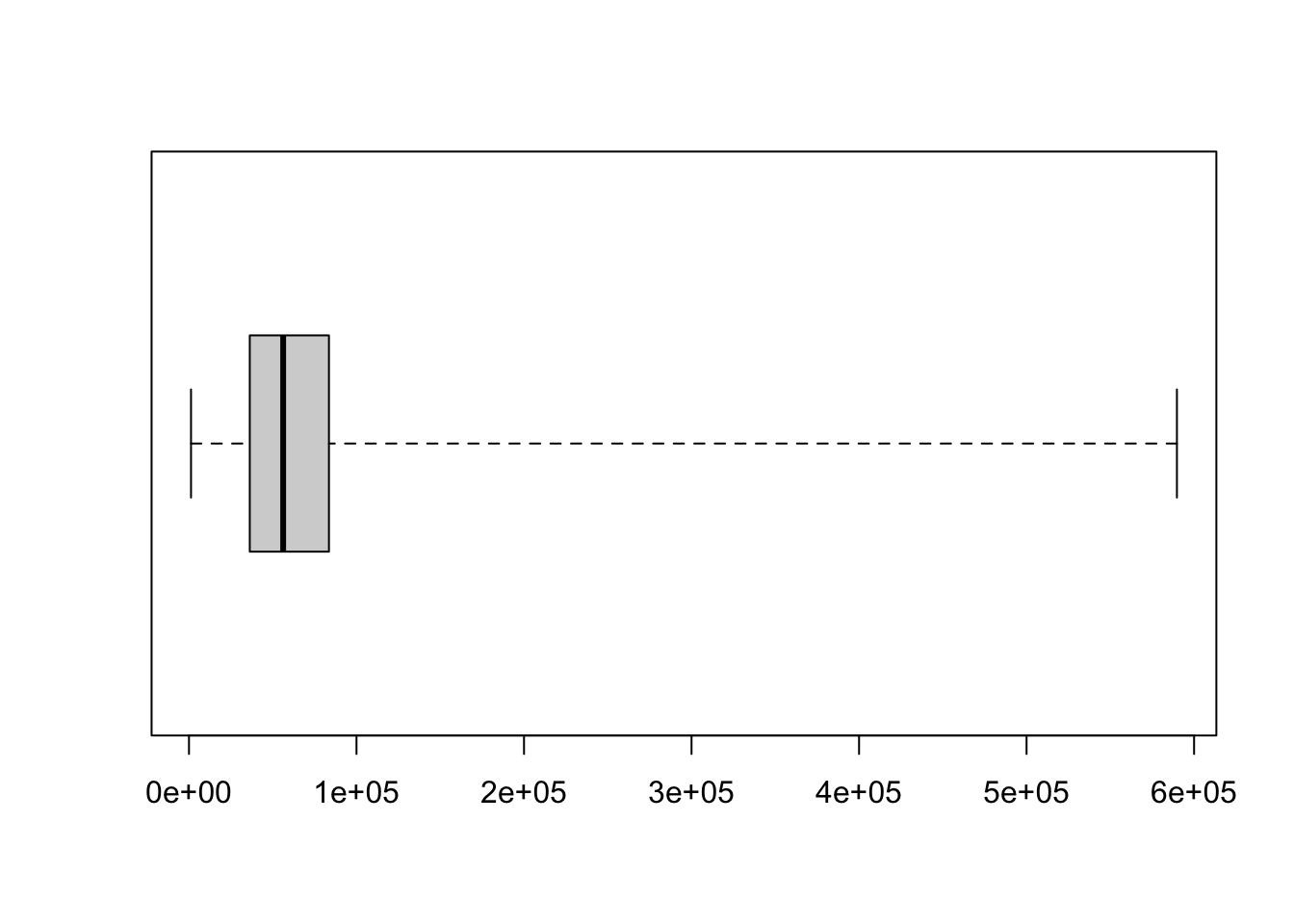
Figure 4.2: Simple Box Plot of state.area
We compare this to the five number summary of state.area which we find via the function fivenum.51
## [1] 1214 36291 56222 83557 589757We remind the reader that the value 1e+05 represents 100,000, 2e+05 represents 200,000, etc. and that the five number summary is the ordered list below.
\[ \text{min}, \;\; Q_1, \;\; \text{Median}, \;\; Q_3, \;\; \text{Max}\]
From this, we see the following.
The left most vertical segment is aligned with \(\text{min} = 1214\).
The left side of the box is aligned with \(Q_1 = 36291\).
The line dividing the box is aligned with \(\text{Median} = 56222\).
The right side of the box is aligned with \(Q_3 = 83557\).
The right most vertical segment is aligned with \(\text{max} = 589575\).
When viewing a box plot, it is helpful to remember that it is dividing a dataset into four parts. Approximately half of the values are within the box (i.e. between \(Q_1\) and \(Q_3\)) where a quarter of all values (or half of the box) are on the left of the median within the box and a quarter of all values (or half of the box) are on the right of the median within the box. There is also roughly a quarter of all values to the left of the box and the remaining quarter of values are to the right of the box. This can be another way to look at the skew of a dataset, which we introduced in Section 3.4. In this example we see a much longer “right tail” and would say the distribution of state areas is right skewed.
4.3.2 (Modified) Box Plots
Some books call the case where range is not specified (or is set to 1.5) a Modified Box Plot. This version of the box plot will show values which can be investigated as Potential Outliers. However, in this book, we will take Box Plot to be the type of graph we construct below.
Example 4.12 The following code shows the box plot for state.area where we omit the option range = 0.

Figure 4.3: (Modified) Box Plot of state.area
This graphically tells us that there are three values which should be considered potential outliers.
Definition 4.11 Given a numeric vector, \(x\), we say that a value is a Potential Outlier if it falls more than one and a half times the interquartile length beyond the interquartile range. That is, if \(\text{IQR}\) is the interquartile range length and \(Q_1\) and \(Q_3\) are the first and third quartiles respectively, then a value is a Potential Outlier if
\[ x < Q_1 - 1.5\cdot \text{IQR} \;\;\text{ or } \;\;x > Q_3 + 1.5\cdot \text{IQR}.\] For simplicity’s sake, we will say that a value that is not a potential outlier is a non-outlier.
The fact that a value is a potential outlier does not mean that it should necessarily be excluded from calculations or graphs. It simply means that the value is a bit atypical of the rest of the data and it should be considered carefully.
You can use the following code chunk to find the potential outliers of a data set x.
Example 4.13 If we set x to be state.area, we get the following.
data <- state.area
#Do not modify the code below this line
PotentialOutliers <- data[
    { data < quantile( data, 1/4, na.rm = TRUE ) - 1.5*IQR( data, na.rm = TRUE) } |
    { data > quantile( data, 3/4, na.rm = TRUE ) + 1.5*IQR( data, na.rm = TRUE) }
   ]
PotentialOutliers
## [1] 589757 158693 267339We see three values that are potential outliers which agrees with our box plot above.
To understand more about the box plot we first saw in Example 4.12, we need the following definitions.
Definition 4.12 The Lower Fence of a box plot of a vector \(x\) is taken to be the smallest non-outlier of the dataset.
The Upper Fence of a box plot of a vector \(x\) is taken to be the largest non-outlier of the dataset.
You can find the lower and upper fences of a vector x along with the set of non-outliers using the following code.
#User must supply the value of x
data <- x
#Do not modify the code below this line
PotentialOutliers <- data[
    { data < quantile( data, 1/4, na.rm = TRUE ) - 1.5*IQR( data, na.rm = TRUE) } |
    { data > quantile( data, 3/4, na.rm = TRUE ) + 1.5*IQR( data, na.rm = TRUE) }
   ]
NonOutliers <- data[ !{data %in% PotentialOutliers} ]  #Removes the Outliers from data
LowerFence <- min(NonOutliers)
UpperFence <- max(NonOutliers)
Any NA values in x will fall into PotentialOutliers and not NonOutliers.
Example 4.14 We illustrate how to use this code using state.area.
data <- state.area
#Do not modify the code below this line
PotentialOutliers <- data[
    { data < quantile( data, 1/4, na.rm = TRUE ) - 1.5*IQR( data, na.rm = TRUE) } |
    { data > quantile( data, 3/4, na.rm = TRUE ) + 1.5*IQR( data, na.rm = TRUE) }
   ]
NonOutliers <- data[ !{data %in% PotentialOutliers} ]  #Removes the Outliers from data
LowerFence <- min(NonOutliers)
UpperFence <- max(NonOutliers)
This shows us that our lower fence is at 1214
## [1] 1214and our upper fence is at 147138.
## [1] 147138This means that the smallest non-outlier is 1,214 (which is also the minimum value) and the largest non-outlier is 147,138.
We can redraw the box plot from above to look at these values in the plot.
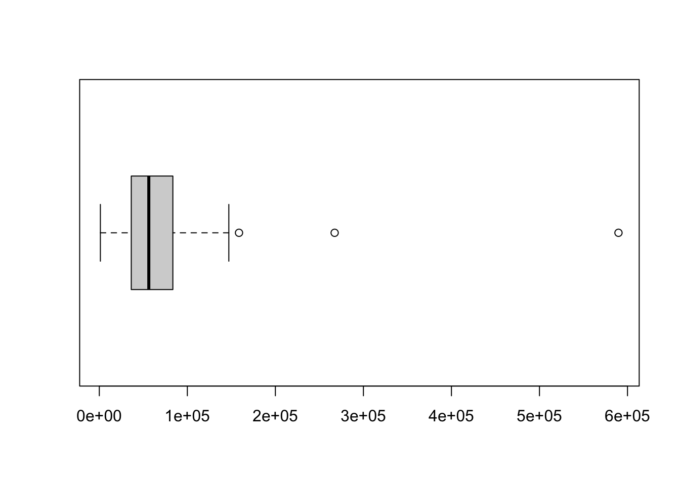
Figure 4.4: Copy of Box Plot of state.area
The Lower Fence is drawn as the vertical line at the left most part of the plot which aligns just to the right of 0e+00 for a value of 1,214. The Upper Fence is drawn as the vertical line which is aligned nearly halfway between 1e+05 and 2e+05 at the value 147,138. The actual box of the boxplot indicates the interquartile range. That is, the left side of the rectangle is at \(Q_1\) and the right side is at \(Q_3\). We also see our three outliers sitting to the right of the upper fence.
Definition 4.13 A Box Plot is a graph where the box is identical to the simple box plots we defined in Definition 4.10 and the extreme left and right vertical segments are aligned with the lower and upper fences respectively and not necessarily the minimum and maximum values. Moreover, any potential outliers are drawn as points (small circles with the default options in R) outside of the fences.
To create a boxplot of a vector, x, you can use the following code
or on the column named ColName of a dataframe named df via the code below.
Many books show box plots in a horizontal fashion rather than vertical. This was done by adding the option horizontal = TRUE. The vertical option will be shown in the following example by removing the horizontal argument.
Example 4.15 The state.area vector we looked at before is an example of a data set where the modified box plot does show potential outliers. If you want the graphs to be shown vertically, we can do that with the following code.
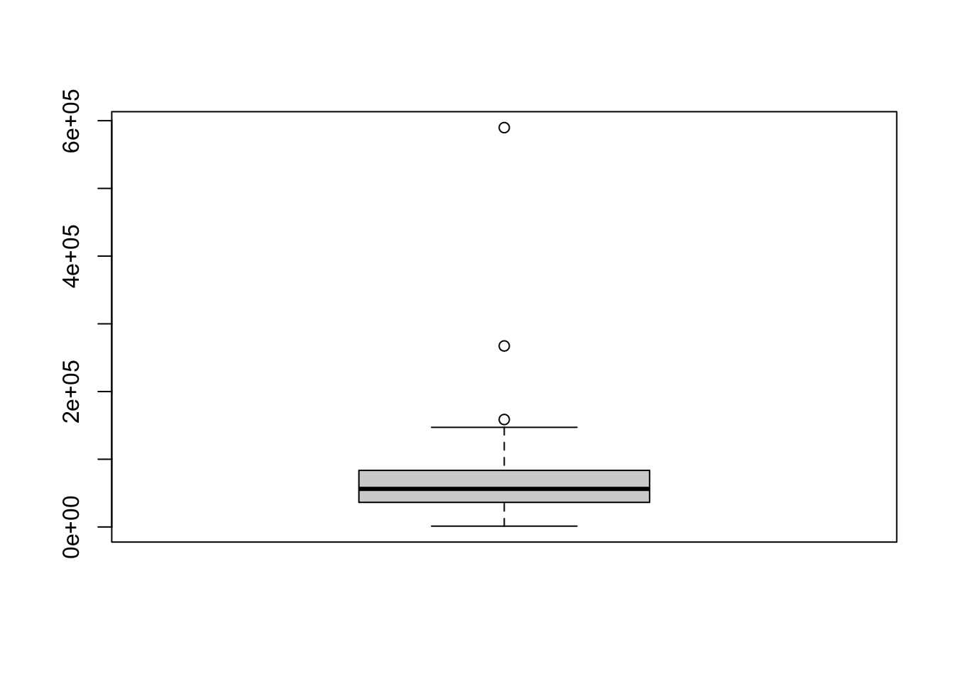
Figure 4.5: Example of a Vertical Box Plot
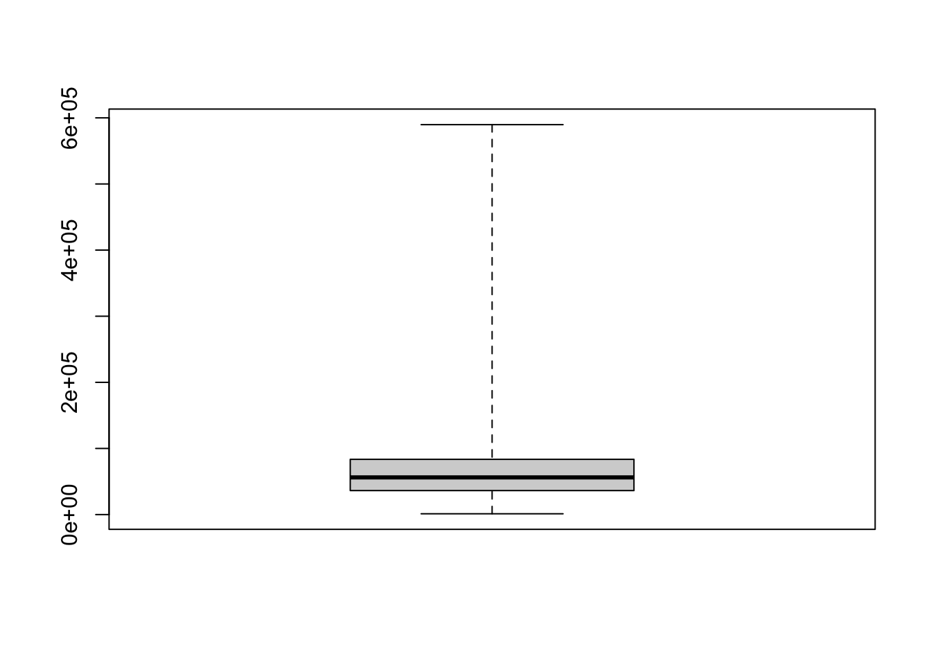
Figure 4.6: Example of a Vertical Simple Box Plot
It is the opinion of the author that horizontal box plots are preferred in most cases. All box plots given as answers to exercises in this document should be given horizontally.
4.4 Measures of Relative Position
We used the quartiles to describe a measure of variability in Section 4.2.3, namely the interquartile range. However, the quartiles by themselves measure something different. The first quartile, \(Q_1\), is a value that is greater than approximately one quarter of all values in the dataset. This is what we will call a Measure of Relative Position. It is often an important question to ask how data values compare to others within the population rather than looking solely at the value alone. For example, is a score of 73 good on an exam? Well, if the mean score was a 48, then that is likely a very good score. However, if the median score was a 78, then that would score lower than more than half of the class. Measures of Relative Position can be used to determine how extreme a data value is among a population or even compare data values from different populations. We will look at a few different measures of relative position in this section.
4.4.1 The quantile function
The five number summary consists of five values: \(Q_0\), \(Q_1\), \(Q_2\), \(Q_3\), and \(Q_4\). We have seen how to use the summary function to find all of the quartiles (as well as the mean) and also have functions to find \({Q_0, Q_2, \text{ and } Q_4}\) directly. Those being min, median, and max respectively. However, we haven’t looked at a function that can find \(Q_1\) or \(Q_3\) by themselves. Quartiles are special cases of quantiles which we will now define.
Definition 4.14 Given a population or dataset and a certain proportion, \(p \in [0,1]\), we can find a value, say \(q\), that separates the data so that at least the proportion \(p\) of the values are no more than \(q\) and at least the proportion \({1-p}\) of the values are no less than \(q\). We call this value \(q\) the Quantile of the data based on \(p\).
Example 4.16 The above definition immediately gives that the median is the quantile of a dataset based on \(p = \frac{1}{2}\) and that the quartiles, \(Q_1\) and \(Q_3\), are the quantiles based on \(p = \frac{1}{4}\) and \(p = \frac{3}{4}\) respectively. That is, the first quartile is the quantile that separates the bottom quarter, or \(p = \frac{1}{4}\), of data values.
Some people find keeping the difference between quartile and quantile clear in their minds. It may be helpful to remember that a QUARTile is used when looking at QUARTers of data and a QUANTile is simply a QUANTity that separates off a certain proportion of values.
We are now ready to look at an R function which will find quantiles for us. It is called, simply enough, quantile().
The syntax of quantile is
where the arguments are
x: The data being considered.probs: A numeric value or vector of probabilities with values in \([0,1]\).
Earlier in Example 4.2 we calculated the median of the fuel efficiencies in the mtcars dataset. We used Definition 4.3 as well as the median function to get the value of 19.2. We can now use the quantile function to see if it agrees with those methods by setting x = mtcars$mpg and probs = 0.5.
##  50%
## 19.2
This shows we have yet another method for finding the median of a dataset.
The quantile() function can be utilized on a vector, x, via
or on the column named ColName of a dataframe named df via
where probs is either a proportion or a vector of proportions. [Each proportion must be between 0 and 1, inclusive.]
Example 4.17 The dataset rivers is built into R and it “gives the lengths (in miles) of 141 ‘major’ rivers in North America, as compiled by the US Geological Survey.” If we wanted to find the third quartile, or \(Q_3\), of this dataset, we can use quantile and set probs = 0.75.
## 75%
## 680
This says that at least 75% of major rivers in North America are no longer than 680 miles.
We will see other quantile functions throughout the book dealing with specific distributions such as the Normal and binomial distributions. These functions will be called qnorm() and qbinom(), where the q literally stands for quantile, respectively and will have the same underlying structure as quantile.
4.4.2 Percentiles
The notation of quantile naturally leads us to consider other proportions other than the ones used in the five number summary. We can ask for the quantile of a dataset based on any percentage and will call this value a percentile. The function quantile can be used to find percentiles.
There is some dispute about the proper way to define percentiles. The \(n\)th percentile is sometimes used to indicate a value such that \(n\)% of all data values will be strictly less than the percentile. We have taken it to mean that \(n\)% of all data values are no more than the percentile.
If we use the definition where there is \(n\)% of values strictly less than the percentile, then it is not possible to be in the 100th percentile as that would imply that an individual, which is in the population, is strictly greater than all values in the population. In this interpretation, it only makes sense to talk about percentages for the integers \(0, 1, 2, \ldots, 99\).
However if we use our interpretation of the percentile than it is possible to be in the 100th percentile, but it is now not possible to be in the 0th percentile.
As a critical consumer of statistics, we may have to ask questions on which definition of the percentile is being given if the distinction is important.
Example 4.18 To find the 97th percentile of the birth mass of babies, we would use the code
##     97%
## 4309.63
This says that 97% of babies in the dataset have a birth mass that is no greater than 4309.63 grams.
While this will only bother more pedantic readers, birth “weight” is recorded here in grams (i.e. mass), rather than a force measurement of a weight. For a deeper dive, see the footnote in Example 5.8 in Section 5.4.
Example 4.19 We can also ask quantile for multiple percentages at once by combining the values into a vector. For example
##      0%     25%     50%     75%    100%
##  907.00 2934.75 3325.00 3629.00 4825.00
is another way of finding the five number summary for the birth mass of babies.
4.4.3 \(z\)-Scores
Another way to discuss relative position is using what is called a \(z\)-Score.
Definition 4.15 Given a population with mean \(\mu\) and standard deviation \(\sigma\), we can define the \(z\)-score, or simply \(z\), of a data value, \(x\) to be \[ z = \frac{x - \mu}{\sigma}.\] We will also call \(z\)-scores the Standardized Value of \(x\).
It is fairly easy to see that a \(z\)-score of 0 occurs exactly when \(x = \mu\) or that the value in question equals the population mean. We can solve the equation in the definition above for \(x\) to allow us to see the converse relationship. \[x = \mu + z \cdot \sigma\]. This quickly shows us that if \(z=1\) then \(x = \mu + \sigma\) or that \(x\) is one (population) standard deviation more than the mean. Similarly, \(z = -2\) gives \(x = \mu - 2 \cdot \sigma\) means that \(x\) is 2 standard deviations less than the mean.
The \(z\)-score a data value is how many population standard deviations it falls above or below the population mean. Positive \(z\)-scores occur for data values greater than the population mean and negative \(z\)-scores occur for data values less than the population mean.
We can use this concept to compare values across different populations.
Example 4.20 In 2022, when she was a high school senior, Linda scored 690 on the mathematics part of the SAT. The distribution of SAT math scores in 2022 had a population mean of 528 and standard deviation of 117. Jake took the ACT and scored 27 on the mathematics portion. ACT math scores for 2022 had a population mean of 20.5 and standard deviation of 5.5.
If we calculate Linda’s \(z\)-score we get the following.
## [1] 1.384615This says that Linda scored approximately 1.38 standard deviations above the mean.
We can now calculate Jake’s standardized value.
## [1] 1.181818This says that Jake scored approximately 1.18 standard deviations above the mean.
While we don’t know the exact distributions of the two populations, SAT scores and ACT scores, we can confidently say that Linda had a score which was more extreme than Jake had. That is, Linda’s score seems to be higher among SAT scores than Jake’s score is among ACT scores.
We will return to this concept in more depth in Chapter 7 when we discuss Normal distributions as well as the Standard Normal Distribution. In that chapter we will be able to make more confident statements about situations like the one we discussed in the above example.
Example 4.21 (Shaq and Britney) Shaquille O’Neal52, also known as Shaq, is a former professional basketball player and widely considered to be a cultural icon. Shaq stands at a staggering 7 foot 1 inch tall, or 85 inches tall. Britney Griner53 is a professional basketball player who has also entered the cultural discussion. Britney stands at 6 foot 9 inches tall, or 81 inches tall. If we ask the “kindergarten” question, “Who is taller?”, the answer is clear that Shaq is taller than Britney. However, a more nuanced question is whether Shaq is taller among men than Britney is among women.
We can use \(z\)-scores to answer this question. The distribution of heights of US adult males has a population mean of \(\mu = 69\) (or 5 foot 9 inches tall) and a population standard deviation of \(\sigma = 3\). This gives us the following for Shaq’s \(z\)-score.
\[z_{\text{Shaq}} = \frac{ 85 - 69 }{3}\] We can also use R to make this calculation as shown below.
## [1] 5.333333This tells us that Shaq occurs 5 and a third population standard deviations above the population mean.
For Britney, the distribution of heights of US adult females has a population mean of \(\mu = 64.5\) (or 5 foot 4.5 inches tall) and a population standard deviation of \(\sigma = 2.5\). This gives us the following for Britney’s \(z\)-score.
\[z_{\text{Britney}} = \frac{ 81 - 64.5 }{2.5}\] We can also use R to make this calculation as shown below.
## [1] 6.6This tells us that Britney occurs 6.6 population standard deviations above the population mean.
As Britney occurs more standard deviations from her population’s distribution, we can conclude that Britney is taller among women than Shaq is among men.
4.5 Resistance
In Section 3.4, we investigated how distributions can be skewed. The skew of a distribution will affect the value of different statistics of a given dataset in different ways. To get a quick feeling of what we mean, we will will return to some of the examples of distributions we saw in Section 3.4.
If we look at a symmetric distributions like the one below, the value of the median (in red) and mean (which is green and directly aligned with the median) both perfectly align with the peak of the distribution.
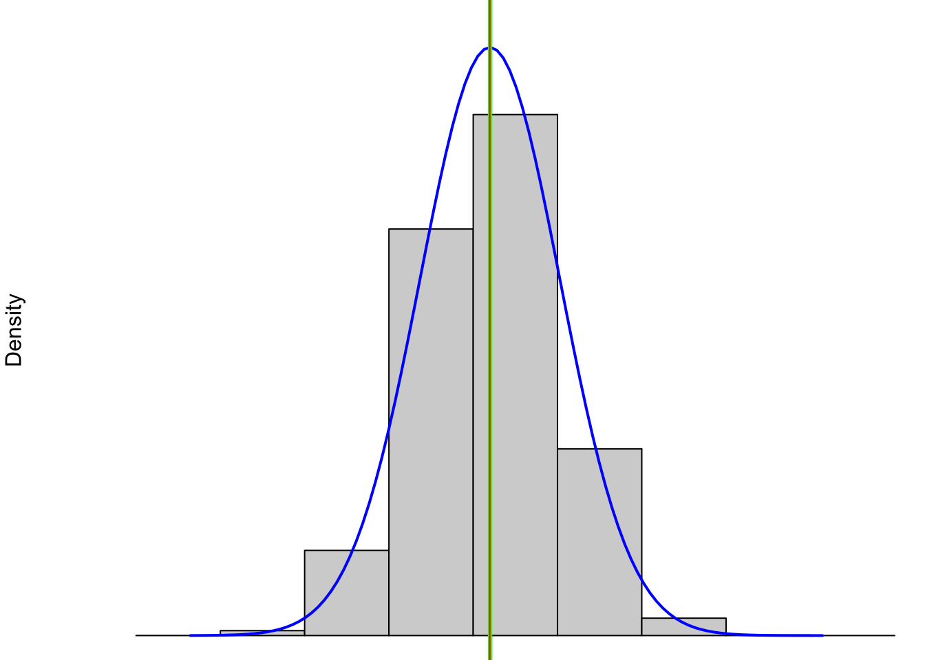
Figure 4.7: Symmetric Distribution
If we shift to a right skewed distribution, as shown below, we see that both of the median (red) and mean (green) have moved away from the peak. The skew has affected both statistics, but it has “pulled” the mean even further in the direction of the skew.
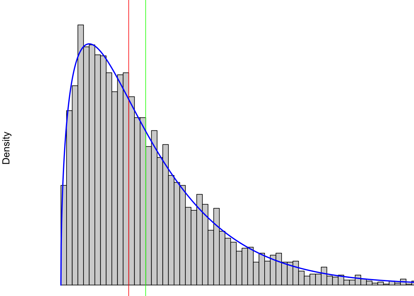
Figure 4.8: Right Skewed Distribution
If we finally look at left skewed data, we see the exact mirror of above. Both statistics are still pulled in the direction of the skew and once again the mean (green) being pulled further to the left than the median (red).
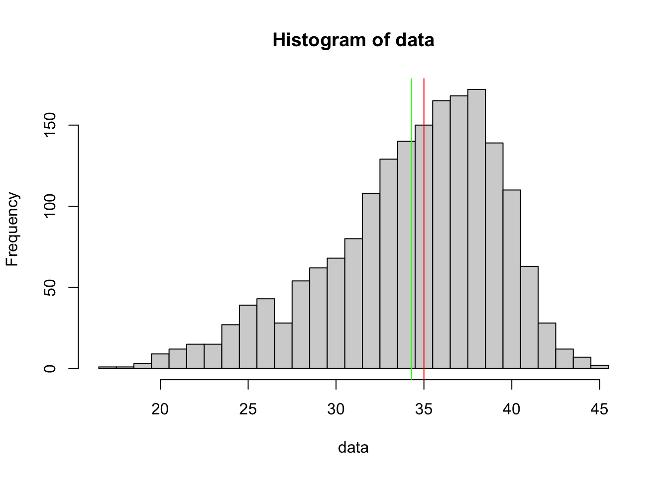
Figure 4.9: Left Skewed Distribution
We will say that a numerical summary is Resistant if skew and extreme values do not have a significant impact on its value.
While we will forego a formal definition, we will make the statement that the following numerical summaries are Resistant:
- median, IQR, \(Q_1\), \(Q_3\)
while the following are Not Resistant:
- mean, standard deviation, range
We can visualize the effects of skew on these statistics with an exploration.
Use the above exploration to create an example of a sample that satisfies the following:
The Mean is greater than the Median.
The Mean is less than the Median.
The Upper Fence does not match the Maximum.
The Interquartile Range is wider than 2 standard deviations.
The Upper Fence falls less than one standard deviation above the mean.
The Minimum is less than one standard deviation below the mean.
Review for Chapter 4
Chapter 4 Quiz: Numerical Summaries of Data
This quiz tests your understanding of core statistical terminology, types of variables, and research methods presented in Chapter 4. The answers can be found prior to the Exercises section.
True or False: The median is a resistant measure of center because its value is not substantially influenced by extreme outliers in the dataset.
True or False: If a data distribution is strongly right-skewed (pulled to the right), the mean will typically be a smaller value than the median.
True or False: The standard deviation is defined as the square of the variance.
True or False: The range is considered a highly resistant measure of spread because it only relies on the maximum and minimum values of the data.
True or False: The interquartile range (IQR) represents the spread of the middle 50% of the data, calculated as the difference between the third quartile, \(Q_3\), and the first quartile, \(Q_1\).
True or False: To identify a potential outlier, the upper fence is calculated by subtracting \(1.5 \cdot \text{IQR}\) from the third quartile, \(Q_3\).
True or False: The standard deviation is a measure of spread that provides an estimate of the average distance of each observation from the mean.
True or False: The function
sd()calculates the population standard deviation, \(\sigma_{\bf x}\).True or False: For any dataset with an odd number of observations, the Median must always be equal to the value of one of the observations in the dataset.
True or False: A simple box plot is a graphical representation of the five number summary.
Definitions
Section 4.1
Definition 4.1 \(\;\) Given a vector \({\bf x} = ( x_1, x_2, \ldots, x_n )\) having \(n\) values, we can define the arithmetic mean or simply mean of \({\bf x}\), which we denote as \(\bar{x}\) if \({\bf x}\) is a sample or \(\mu\) if \({\bf x}\) is the entire population, as follows. \[\bar{x} \text{ or }\mu= \frac{1}{n} \sum_{i = 1}^n x_i = \frac{1}{n} \left( x_1 + x_2 + \cdots + x_n \right) = \frac{ x_1 + x_2 + \cdots + x_n }{n}.\]
Definition 4.2 \(\;\) The Deviation of a Value, \(x_i\), of a vector \({{\bf x} = ( x_1, x_2, \ldots, x_n)}\), is defined as \[ \text{dev}(x_i) = x_i - \bar{x}\] or \[ \text{dev}(x_i) = x_i - \mu.\] We define the Deviation of a Vector to be the vector of its deviations. That is,
\[\text{dev}({\bf x}) = \left(\text{dev}(x_1), \text{dev}(x_2), \ldots, \text{dev}(x_n) \right).\]
Definition 4.3 \(\;\) Let \({\bf x}\) be a vector of \(n\) values, \((x_1, x_2, \ldots, x_n)\). We can reorder them and (possibly) relabel them as \((w_1, w_2, \ldots, w_n)\) such that \(w_1 \leq w_2 \leq \cdots \leq w_n\) and each \(w_i\) is some \(x_j.\) We can define the the Median of \({\bf x}\) based on the parity of \(n\), i.e. whether it is even or odd.
If \(n\) is odd, then let \(L = \frac{n-1}{2}\) (which means \(n = 2L + 1\)) and we define the Median of \(x\) to be \(w_{L+1}\).
If \(n\) is even, then let \(K = \frac{n}{2}\) (which means that \(n = 2K\)) and we define the Median of \({\bf x}\) to be the value \(\frac{w_K + w_{K+1}}{2}\), or the arithmetic mean of the two most “middle” values of \({\bf x}\).
Section 4.2
Definition 4.4 \(\;\) Given a finite list of quantitative values, \(x\), we define the Range of \(x\) to be the interval \([ \text{min}, \text{Max}]\) where \(\text{min}\) is the minimum value of \(x\) and \(\text{Max}\) is the maximum value.
Definition 4.5 \(\;\) If a dataset has a range of \([\text{min}, \text{Max}]\), then the Range Length is defined to be the value \(\text{Max}-\text{min}\).
Definition 4.6 \(\;\) For \(k =0,1,2,3,4\), the \(k\)th Quartile, \(Q_k\) is a number such that at least the proportion \(\frac{k}{4}\) of the values in the dataset are no more than \(Q_k\) and at least the proportion \(1-\frac{k}{4}\) of the values are no less than \(Q_k\). We also require that \(Q_2\) is the median of the dataset (as defined in Definition 4.3) and that \(Q_0\) and \(Q_4\) are \(\text{min}\) and \(\text{Max}\) (as defined in Definition 4.4) respectively.
Definition 4.7 \(\;\) The Interquartile Range of a dataset is defined to be the interval \([Q_1, Q_3]\). We also define the Interquartile Range Length to be the value \(Q_3 - Q_1\).
Definition 4.8 \(\;\) Given a vector \({\bf x} = ( x_1, x_2, \ldots, x_n )\) having \(n\) values (with \(n\geq 2\)), we can define the Sample Standard Deviation of \({\bf x}\), denoted by \(s_{\bf x}\), to be
\[ s_{\bf x} = \sqrt{ \frac{\displaystyle{\sum \left( x_i - \bar{x}\right)^2}}{n-1}}.\] We can also define the Sample Variance to be the square of the sample standard deviation. That is, the sample variance is \[ s_{\bf x}^2 = \frac{\displaystyle{\sum \left( x_i - \bar{x}\right)^2}}{n-1}.\]
Definition 4.9 \(\;\) Given a population \({\bf x} = ( x_1, x_2, \ldots, x_N )\) having \(N\) values (with \(N\geq 2\)), we can define the Population Standard Deviation of \({\bf x}\), denoted by \(\sigma_{\bf x}\), to be
\[ \sigma_{\bf{x}} = \sqrt{ \frac{\displaystyle{\sum \left( x_i - \bar{x}\right)^2}}{N}}.\] We can also define the Population Variance to be \[ \sigma_{\bf{x}}^2 = \frac{\displaystyle{\sum \left( x_i - \bar{x}\right)^2}}{N}.\]
Section 4.3
Definition 4.10 \(\;\) A Simple Box Plot is a graph that illustrates the five number summary. A vertical segment is drawn above the value of the minimum as well as the maximum. A box is then created with its left side aligning with \(Q_1\) and its right side aligning with \(Q_3\). The median is indicated by a vertical line within the box which divides the box into 2 parts. The box is then connected to the left and right segments with dashed lines which are often called whiskers.
Definition 4.11 \(\;\) Given a numeric vector, \(x\), we say that a value is a Potential Outlier if it falls more than one and a half times the interquartile length beyond the interquartile range. That is, if \(\text{IQR}\) is the interquartile range length and \(Q_1\) and \(Q_3\) are the first and third quartiles respectively, then a value is a Potential Outlier if
\[ x < Q_1 - 1.5\cdot \text{IQR} \;\;\text{ or } \;\;x > Q_3 + 1.5\cdot \text{IQR}.\] For simplicity’s sake, we will say that a value that is not a potential outlier is a non-outlier.
Definition 4.12 \(\;\) The Lower Fence of a box plot of a vector \(x\) is taken to be the smallest non-outlier of the dataset.
The Upper Fence of a box plot of a vector \(x\) is taken to be the largest non-outlier of the dataset.
Definition 4.13 \(\;\) A Box Plot is a graph where the box is identical to the simple box plots we defined in Definition 4.10 and the extreme left and right vertical segments are aligned with the lower and upper fences respectively and not necessarily the minimum and maximum values. Moreover, any potential outliers are drawn as points (small circles with the default options in R) outside of the fences.
Section 4.4
Definition 4.14 \(\;\) Given a population or dataset and a certain proportion, \(p \in [0,1]\), we can find a value, say \(q\), that separates the data so that at least the proportion \(p\) of the values are no more than \(q\) and at least the proportion \({1-p}\) of the values are no less than \(q\). We call this value \(q\) the Quantile of the data based on \(p\).
Definition 4.15 \(\;\) Given a population with mean \(\mu\) and standard deviation \(\sigma\), we can define the \(z\)-score, or simply \(z\), of a data value, \(x\) to be \[ z = \frac{x - \mu}{\sigma}.\] We will also call \(z\)-scores the Standardized Value of \(x\).
Big Ideas
Section 4.2
The Standard Deviation is a measure of spread that provides an estimate of the average distance of each observation from the mean.
The standard deviation is never negative and 0 exactly when all the values of a dataset are identical.
Section 4.4
The \(z\)-score a data value is how many population standard deviations it falls above or below the population mean. Positive \(z\)-scores occur for data values greater than the population mean and negative \(z\)-scores occur for data values less than the population mean.
Section 4.5
While we will forego a formal definition, we will make the statement that the following numerical summaries are Resistant:
- median, IQR, \(Q_1\), \(Q_3\)
while the following are Not Resistant:
- mean, standard deviation, range
Important Alerts
Section 4.1
Quartile calculations can be done in many ways and using summary() and IQR() will not always agree. There are functions in the appendix of this chapter that will give versions which will agree with a lot of other introductory statistics textbooks.
Unless we explicitly say we are looking at a population standard deviation, we will assume that the phrase standard deviation means a sample standard deviation throughout Statypus.
The fact that a value is a potential outlier does not mean that it should necessarily be excluded from calculations or graphs. It simply means that the value is a bit atypical of the rest of the data and it should be considered carefully.
Section 4.4
There is some dispute about the proper way to define percentiles. The \(n\)th percentile is sometimes used to indicate a value such that \(n\)% of all data values will be strictly less than the percentile. We have taken it to mean that \(n\)% of all data values are no more than the percentile.
If we use the definition where there is \(n\)% of values strictly less than the percentile, then it is not possible to be in the 100th percentile as that would imply that an individual, which is in the population, is strictly greater than all values in the population. In this interpretation, it only makes sense to talk about percentages for the integers \(0, 1, 2, \ldots, 99\).
However if we use our interpretation of the percentile than it is possible to be in the 100th percentile, but it is now not possible to be in the 0th percentile.
As a critical consumer of statistics, we may have to ask questions on which definition of the percentile is being given if the distinction is important.
Important Remarks
Section 4.1
While some statistics courses also discuss the mode in conjunction with the median and mean, it is not a measure of central tendency. In fact, it is quite possible for the mode to be either the minimum or maximum value of a dataset.
It is important to make a distinction between a population mean, denoted as \(\mu\), which is a parameter and a sample mean, denoted \(\bar{x}\), which is a statistic. Often, we are unable to work with an entire population, so we will often be using a sample to calculate \(\bar{x}\) which will be our best guess for \(\mu\). As mentioned in Chapter 2, this will be a common thread throughout our work. We will often default to denoting a mean as \(\bar{x}\) when working with data as often we will only be able to work with a sample of a population.
Section 4.2
In this book, we will adopt the convention to call any group of numbers, \(Q_k\) for \(k = 0,1,2,3,4\), that satisfies Definition 4.6 a “Five Number Summary.”
- A lot of books define the interquartile range to be what we have called the interquartile range length. We have chosen this notation to make it consistent with that of range.
- We may blur between the interquartile range and the interquartile range length and hope that context will make the situation clear.
- Due to our lack of uniqueness in defining \(Q_1\) and \(Q_3\), there is some ambiguity in our definition of both the interquartile range and the interquartile range length. In practice, simply supplying the code used to make a calculation will remove this issue.
- Like with the mean, we use Greek letters (\(\mu\) and \(\sigma\)) to represent population parameters and Roman or Latin letters (\(\bar{x}\) and \(s\)) to represent sample statistics. As we will see in later chapters, we will be using statistics to approximate parameters.
- We will rarely work with variances directly, but the concept will appear in a few later chapters of Statypus.
Section 4.3
When viewing a box plot, it is helpful to remember that it is dividing a dataset into four parts. Approximately half of the values are within the box (i.e. between \(Q_1\) and \(Q_3\)) where a quarter of all values (or half of the box) are on the left of the median within the box and a quarter of all values (or half of the box) are on the right of the median within the box. There is also roughly a quarter of all values to the left of the box and the remaining quarter of values are to the right of the box. This can be another way to look at the skew of a dataset, which we introduced in Section 3.4. In this example we see a much longer “right tail” and would say the distribution of state areas is right skewed.
Section 4.4
Some people find keeping the difference between quartile and quantile clear in their minds. It may be helpful to remember that a QUARTile is used when looking at QUARTers of data and a QUANTile is simply a QUANTity that separates off a certain proportion of values.
Code Templates
Section 4.1
The function mean() can be utilized on a vector, x, via
or on the column named ColName of a dataframe named df via
Section 4.2
The range function can be utilized on a vector, x, via
or on the column named ColName of a dataframe named df via
This summary function can be utilized on a vector, x, via
or on the column named ColName of a dataframe named df via
If you run
on a data frame, df, it will return the result of summary for each column. The results for non-quantitative variables may yield varied results.
Section 4.3
To plot a simple box plot, you can use the following code template.
or
You can use the following code chunk to find the potential outliers of a data set x.
You can find the lower and upper fences of a vector x along with the set of non-outliers using the following code.
#User must supply the value of x
data <- x
#Do not modify the code below this line
PotentialOutliers <- data[
    { data < quantile( data, 1/4, na.rm = TRUE ) - 1.5*IQR( data, na.rm = TRUE) } |
    { data > quantile( data, 3/4, na.rm = TRUE ) + 1.5*IQR( data, na.rm = TRUE) }
   ]
NonOutliers <- data[ !{data %in% PotentialOutliers} ]  #Removes the Outliers from data
LowerFence <- min(NonOutliers)
UpperFence <- max(NonOutliers)Section 4.4
The quantile() function can be utilized on a vector, x, via
or on the column named ColName of a dataframe named df via
where probs is either a proportion or a vector of proportions. [Each proportion must be between 0 and 1, inclusive.]
New Functions
Section 4.1
The syntax of mean is
where the argument is
na.rm: A logical ofTRUEorFALSEindicating whetherNAvalues should be stripped before the computation proceeds.
Section 4.2
The syntax of min is
where the argument is
na.rm: A logical ofTRUEorFALSEindicating whetherNAvalues should be stripped before the computation proceeds.
The syntax of max is
where the argument is
na.rm: A logical ofTRUEorFALSEindicating whetherNAvalues should be stripped before the computation proceeds.
The syntax of range is
where the argument is
na.rm: A logical ofTRUEorFALSEindicating whetherNAvalues should be stripped before the computation proceeds.
The syntax of summary is
where the argument is
object: An object for which a summary is desired.
The syntax of IQR is
where the argument is
na.rm: A logical ofTRUEorFALSEindicating whetherNAvalues should be stripped before the computation proceeds.
The syntax of sd is
where the argument is
na.rm: A logical ofTRUEorFALSEindicating whetherNAvalues should be stripped before the computation proceeds.
You can also create a new function, which we have called popSD, with the following code:
#This code will load popSD into your environment
popSD <- function( x ){
  sd( x ) * sqrt( ( length( x ) - 1 ) / length( x ) )
  }
This is the formula one would use if they wanted to find the population standard deviation of a finite data set. You must first run the above code before you can use the function.
Section 4.3
The syntax of boxplot is
where the argument is
range: See?boxplotfor a full description. We will userangeonly when we wish to not indicate potential outliers. Settingrange = 0turns off the check of outliers.horizontal: Alogicalvalue indicating if the boxplots should be horizontal; the default isFALSEand results in means vertical boxes.
Section 4.4
Quiz Answers
- True
- False (The Mean is pulled toward the tail, so Mean > Median for right-skewness.)
- False (The Standard Deviation is the square root of the Variance.)
- False (It is highly non-resistant because the two most extreme values dictate the entire measure.)
- True
- False (You add \(1.5 \times \text{IQR}\) to \(Q_3\) for the upper fence.)
- True
- False (The Base R
sd()function calculates the sample standard deviation, \(s\).) - True
- True
Exercises
For Exercises 4.2 through 4.4, you will need to load the dataset hot_dogs. The code for this can be found in Example 1.15.
For Exercises 4.7 and 4.8, you will need to load the dataset BabyData1. The code for this can be found in Example 4.1.
Exercise 4.1 For each of the following parts, identify where the student went wrong and find a way to fix their code. Feel free to run the code as it is to see what Errors or Warnings appear.
- A student tried to find the mean of the dataset
riversusing the following code.
- A student tried to find the median of the dataset
riversusing the following code.
- A student used the following line of code to try and find the \(z\)-score for an IQ score of 73. We know that IQ scores have \(\mu = 100\) and \(\sigma = 15\).
- After successfully loading the
BabyData1data frame as done in Example 4.1, a student used the following code to try to find the range of thedad_agevariable.
Exercise 4.2 Make a box plot of the sodium variable of hot_dogs. Do there appear to be any outliers?
Exercise 4.3 Consider the sodium variable for the hot dogs where the type is Meat. This data has a potential outlier. Produce both a box plot that shows potential outliers and one where the fences go to the max and min values.
Exercise 4.4 Find the summary as well as a box plot for the calories variable in hot_dogs for each type. [You should have 3 summary outputs as well as 3 box plots for this problem.]
Exercise 4.5 Find the mean value of the wt variable for the mtcars dataset. Also find the mean for cars based on the number of cylinders it has. That is, find the mean of the wt variable for each of the possible values of cyl. There should be four total means calculated. What relationship is there between the number of cylinders and the weight of a car?
Exercise 4.6 Find the standard deviation of the mpg variable for the mtcars dataset. Also find the standard deviation for cars based on the number of cylinders it has. There should be four total standard deviations calculated. Which type of engine, based on number of cylinders, has the most and least variability?
Exercise 4.7 Using BabyData1, what are the 1st and 99th percentile of birth masses? Interpret these values.
Exercise 4.8 Quintiles can be defined similarly to quartiles and break a dataset into five equally sized groups. Find the quintiles for the length of gestation in the BabyData1 dataframe. [You should have six different values or five different regions.]
4.6 Appendix
A lot of introductory statistics books define the first quartile to be the median of the lower half of the data set with the median removed and the third quartile analogously. If you want to find results to agree with these definitions, then the following function should resolve possible issues.
QuartileBook <- function(DataArray) {
    x <- sort(DataArray)
    n <- length(x)
    m <- (n+1)/2
    if (floor(m) != m) {
        l <- m-1/2; u <- m+1/2
    } else {
        l <- m-1; u <- m+1
    }
    c(Minimum=min(x),Q1=median(x[1:l]),
      Median=median(x),Q3=median(x[u:n]),
      Maximum=max(x))
}
The following code is a function which returns the IQR of a vector using this definition.
IQRBook <- function(DataArray) {
    x <- sort(DataArray)
    n <- length(x)
    m <- (n+1)/2
    if (floor(m) != m) {
        l <- m-1/2; u <- m+1/2
    } else {
        l <- m-1; u <- m+1
    }
    return(median(x[u:n]) - median(x[1:l]))
}
The following function will find the values in a vector which are outliers under this possibly different definition of IQR.
OutliersBook <- function(DataArray){
    x <- sort(DataArray)
    n <- length(x)
    m <- (n+1)/2
    if (floor(m) != m) {
        l <- m-1/2; u <- m+1/2
    } else {
        l <- m-1; u <- m+1
    }
    x[(x < median(x[1:l])-1.5*(median(x[u:n]) - median(x[1:l]))) |
        (x > median(x[u:n])+1.5*(median(x[u:n]) - median(x[1:l])))]
}
The following code is the sister function to OutliersBook and returns only the values which are not outliers.
TrimBook <- function(DataArray){
    x <- sort(DataArray)
    n <- length(x)
    m <- (n+1)/2
    if (floor(m) != m) {
        l <- m-1/2; u <- m+1/2
    } else {
        l <- m-1; u <- m+1
    }
    x[(x > median(x[1:l])-1.5*(median(x[u:n]) - median(x[1:l]))) &
        (x < median(x[u:n])+1.5*(median(x[u:n]) - median(x[1:l])))]
}
The following code will run the OutliersBook function on each column of a dataframe.
OutliersFrame <- function(DataArray){
    apply(DataArray,2, function(DataArray){
        x <- sort(DataArray)
        n <- length(x)
        m <- (n+1)/2
        if (floor(m) != m) {
            l <- m-1/2; u <- m+1/2
        } else {
            l <- m-1; u <- m+1
        }
        (DataArray < median(x[1:l])-1.5*(median(x[u:n]) - median(x[1:l]))) |
            (DataArray > median(x[u:n])+1.5*(median(x[u:n]) - median(x[1:l])))
    }
    )
}
Stannard, Hayley J.; Old, Julie M. (2023). “Wallaby joeys and platypus puggles are tiny and undeveloped when born. But their mother’s milk is near-magical”. The Conversation.↩︎
While we forego the technical definitons of minimum and maxium wihtin the text, the curious reader may be curious if more care is needed. The most general definition we offer is that \(\text{min}\) is the greatest lower bound of the dataset while \(\text{max}\) is the least upper bound. This allows a generalization to even datasets with infinite data points.↩︎
We do not go into much detail with
fivenumin this book. See?fivenumfor more details.↩︎