Chapter 12 Inference on a Linear Regression

Figure 12.1: A Statypus Having a Torus Pastry

Platypuses are warm blooded, but their average body temperature is \(9^\circ\)F (\(5^\circ\) C) lower than placental mammals like humans. While humans expect a body temperature of \(98.6^\circ\)F (\(37^\circ\)C), a platypus will average \(89.6^\circ\)F (\(32^\circ\)C).¹⁴⁷

In Chapter 5, we investigated the relationship between two quantitative variables, \(x\) and \(y\), using correlation and the least squares regression line. In that chapter, we declared that

\[\hat{y}|_{x = x_0}\] was the mean of all values of \(y\) when \(x = x_0\). However, as this came from a sample, we are quite certain that this value is only a point estimate of the actual population mean of the distribution of \(y\) values such that \(x = x_0\). That is, we can use the concepts introduced in Chapter 9 and then expanded to means in Chapter 10 to conduct inference on our least squares regression line. We will be able to give confidence intervals for the mean discussed above and also make inferences about how much correlation the underlying populations actually have. Using the terminology of Section 10.2.4, we will be able to give Prediction Intervals as well as Confidence Intervals for \(\mu_y\) for any particular value of \(x = x_0\).

New R Functions Used

• rhoConfInt(): Used to estimate the confidence interval for \(\rho\). [Statypus Original Function]

• cor.test(): Test for association between paired samples using Pearson’s product moment correlation coefficient.

• RegressionInference(): Gives confidence intervals for both the \(\hat{y}\) model as well as for values of form \(\hat{y}|_{x = x_0}\).[Statypus Original Function]

Remark. The functions rhoConfInt() and RegressionInference() were developed at Saint Louis University and do not have any built in help files. Please contact Dr. Phil Huling at phil.huling@slu.edu if you have further questions about their functionality.

12.1 Inference on the Correlation Coefficient

In Section 5.3, we defined the Correlation Coefficient based on samples. As such, the formula given there is a statistic which approximates a yet undefined parameter. We remedy this with the following definition.

Definition 12.1 Given two variables, the Population Correlation Coefficient is denoted by \(\rho\) and is a parameter that satisfies the same conditions as \(r\) in Theorem 5.1.

The value of \(r\) defined in Section 5.3 is the statistic or Sample Correlation Coefficient and is a point estimate for \(\rho\) based on a sample of the respective populations.¹⁴⁸

Here at Statypus, we have decided to use the Greek letter \(\rho\), pronounced the same as “row,” for the parameter associated to Pearson’s (Product Moment) Correlation Coefficient. Other sources may not use this notation and it is important to mention that \(\rho\) is also often associated with a different concept of correlation, called Spearman’s Rank Correlation Coefficient or simply Spearman’s \(\bf{\rho}\).¹⁴⁹

Example 12.1 We revisit the ToyCars dataset that we first introduced in Chapter 3 (Example 5.6 to be precise).

ToyCars <- read.csv( "https://statypus.org/files/ToyCars.csv" )

The dataframe contains the height at which a toy car was released down a sloped tube as well as the lateral distance that the car traveled when it left the tube. My children hypothesized that the car would travel further if it was started at a higher point. We can look at the data below.

plot( x = ToyCars$Height, y = ToyCars$Distance )

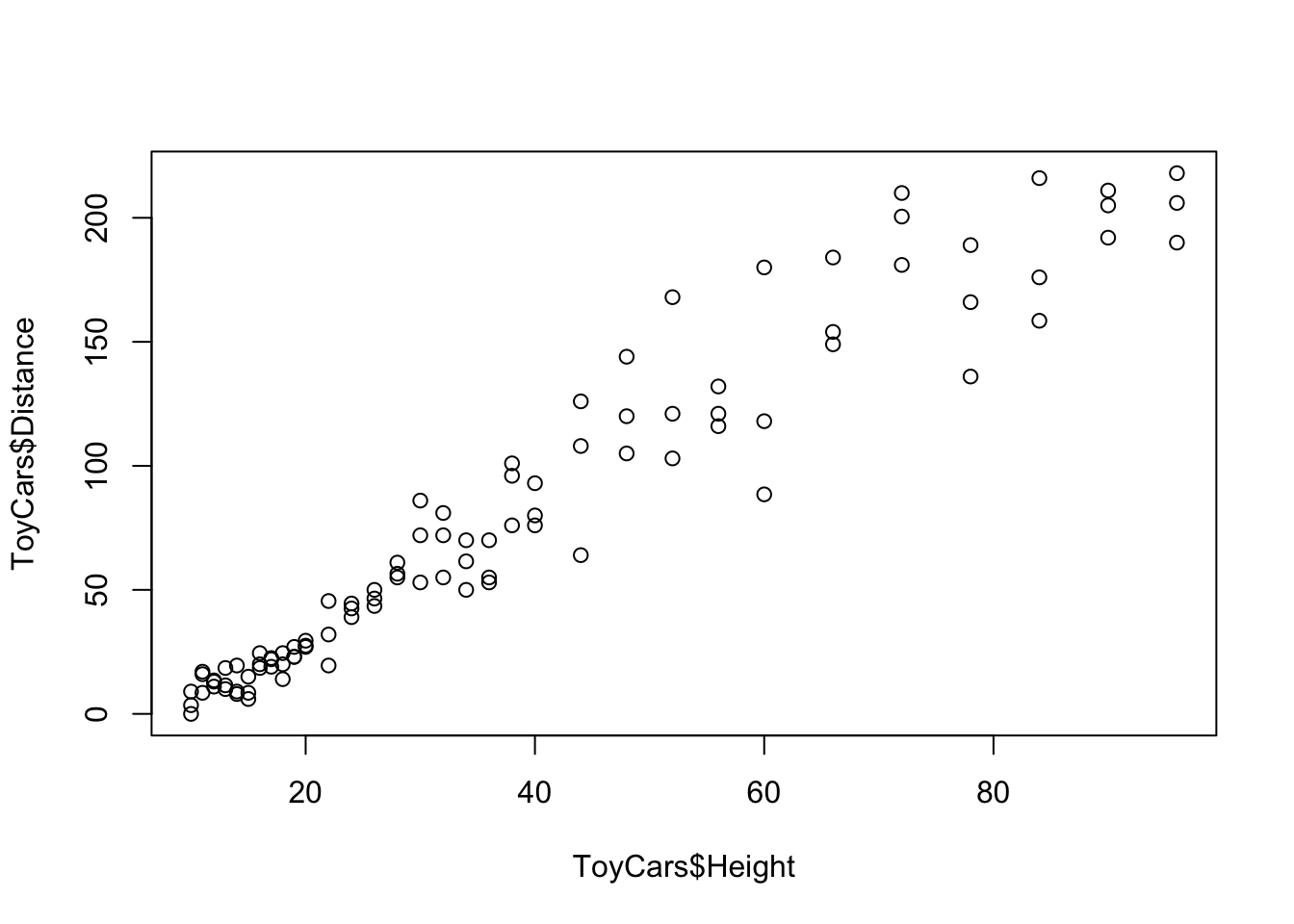
Figure 12.2: Scatterplot of ToyCars

Visually we see a very clear correlation between the Height and Distance variables. To find the correlation coefficient, we use the cor() function introduced in Section 5.3.

cor( x = ToyCars$Height, y = ToyCars$Distance )

## [1] 0.9644005

This means that our point guess for the population correlation coefficient would be 0.9644005. However, this is just a statistic arising from a single sample and as such is nearly certainly not exact.

Therefore, we need to understand the distribution of values of \(r\) in order to be able to discuss a confidence interval for \(\rho\).

Like we did in Chapters 9, 10, and 11 we can look at the distribution of the values of the statistic to make inferences about the parameter. That is, we will look at the distribution of values of \(r\) to make inferences about \(\rho\).

12.1.1 Confidence interval for \(\rho\)

While it is quite possible to develop a model for the distribution of \(r\) values, we will use a new concept here called Bootstrapping.

Definition 12.2 The method of Bootstrapping¹⁵⁰ is to select numerous new (re)samples (i.e. samples using replacement) of a given fixed sample to gain understanding about the distribution that the sample’s statistic lives in.

We will use the concept of bootstrapping to get an approximation for a confidence interval for \(\rho\) based on our sample data. To do this, we will automate the work in a new function, developed at Statypus, called rhoConfInt().

The syntax of rhoConfInt() is

rhoConfInt( x, y, conf.level, size )   
#This code will not run unless the necessary values are inputted.

where the parameters are:

• x, y: Numeric vectors of data values.

• conf.level: The confidence level for the desired confidence interval. Defaults to 0.95.

• size: The number of shuffled samples used to create the confidence interval. Defaults to 10000.

What rhoConfInt does is selects a large number (defined by size which defaults to 10000) of samples of the same size as our sample by selecting (with replacement) \(n\) ordered pairs from our original sample of size \(n\). (This clearly shows why we need replacement, as otherwise all samples would match our original sample.)

We are using the concept that all we really know about the populations is what is contained in the sample, so we attempt to make more samples to see how they vary.

Remark. Methods such as this involve drawing random values and as such will change each time they are run. If you run the code in the example below, you will likely not get the exact same values, but your answer shouldn’t be too far off from it either.

Example 12.2

rhoConfInt( x = ToyCars$Height, y = ToyCars$Distance )

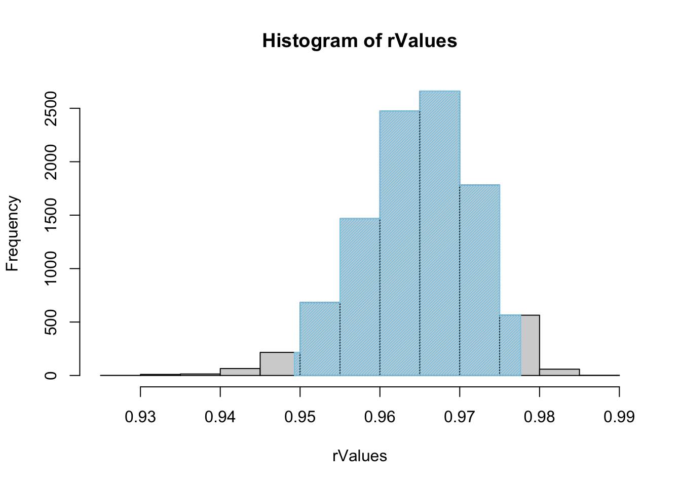
Figure 12.3: Histogram of Shuffled r Values

## $`Confidence Level`
## [1] 0.95
## 
## $`Confidence Interval`
##      2.5%     97.5% 
## 0.9492910 0.9776261 
## 
## $`How Many Shuffles`
## [1] 10000

We can also demand a larger selection of sample by changing the value of size. Here we crank it up to one million to see what happens.

The following block of code may take a fairly long time to run if you try to do it on your own computer.

rhoConfInt( x = ToyCars$Height, y = ToyCars$Distance, size = 1000000 )

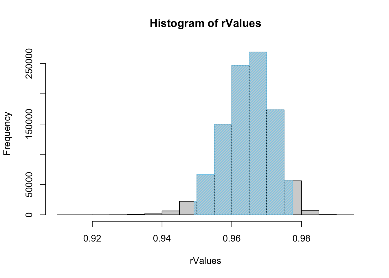
Figure 12.4: Histogram of Shuffled r Values

## $`Confidence Level`
## [1] 0.95
## 
## $`Confidence Interval`
##      2.5%     97.5% 
## 0.9491534 0.9774889 
## 
## $`How Many Shuffles`
## [1] 1e+06

This shows that it appears that setting size as high as one million does not offer much improvement over the default value of 10000 as our values have not changed to 3 decimal places. Going from the default setting to size = 1000000 will also take 100 times the computing time, which is a trade off that may not be worth it if we don’t gain much more information.

This leaves us with the impression that we expect that \(\rho\) is between about 0.9492 and 0.9774.

As before, there is an R function that will automate a lot of this work for us (and do it better). While it won’t offer a picture to analyze like rhoConfInt, the function cor.test() is very strong and actually uses better techniques to produce confidence intervals. It will also have output in a form we are accustomed to by this point.

The syntax of cor.test() is

cor.test( x, y, alternative, conf.level )   
#This code will not run unless the necessary values are inputted.

where the parameters are:

• x, y: Numeric vectors of data values. x and y must have the same length.

• alternative: The symbol in the alternative hypothesis in a hypothesis test. Must be one of "two.sided", "less", and "greater". DO NOT USE for confidence intervals.

• conf.level: The confidence level for the desired confidence interval. Not needed for hypothesis test.

Note: alternative is set to "two.sided" by default if you do not enter this parameter.

The function cor.test is actually more robust than the treatment it will receive here. It can use Pearson’s product moment coefficient (what we called \(r\)), Kendall’s \(\tau\), or Spearman’s \(\rho\).

Example 12.3 We can revisit the ToyCars dataset and now invoke cor.test to find a confidence interval for \(\rho\). The default call of cor.test will give us a 95% confidence interval.

cor.test( x = ToyCars$Height, y = ToyCars$Distance )

## 
##  Pearson's product-moment correlation
## 
## data:  ToyCars$Height and ToyCars$Distance
## t = 35.358, df = 94, p-value < 2.2e-16
## alternative hypothesis: true correlation is not equal to 0
## 95 percent confidence interval:
##  0.9470196 0.9761492
## sample estimates:
##       cor 
## 0.9644005

This gives that we can be 95% confident that \(\rho\) is between 0.947 and 0.976 which matches reasonable well with our bootstrap method in Example 12.2.

Using the dataset BabyData1 which can be downloaded below, find a 98% confidence interval for the population correlation coefficient between the age of a newborn’s mother and the age of the newborn’s father.

BabyData1 <- read.csv( "https://statypus.org/files/BabyData1.csv" )

12.1.2 Hypothesis Test for \(\rho\)

We now turn our gave towards the concept of a hypothesis test. While the techniques used here can be done for more general testing, we will focus on the case when we test if \(\rho = 0\). That is, we wish to see if there is any (linear) correlation between two populations.

To test if there is ANY (linear) correlation between two populations, we can test if the population correlation coefficient, \(\rho\), is not 0.

\[\begin{align*} H_0: \rho &= 0\\ H_a: \rho &\neq 0 \end{align*}\]

We can also test if there is true positive or negative correlation coefficient where the alternative hypothesis is \(H_a: \rho > 0\) or \(H_a: \rho < 0\) respectively.

As compared to our method in Section 12.1.1, we will now give and use information about the distribution of values of \(r\) coming from samples of size \(n\).

Definition 12.3 The Standard Error of \(\bf r\), denoted \(s_r\), based on a sample is a point estimate to the standard deviation of the distribution of sample correlation coefficients, denoted \(\sigma_r\), and is given by \[ \sigma_r \approx s_r = \sqrt{\frac{1-r_0^2}{n - 2}}\] where \(n\) is the size of the sample and \(r_0\) is the sample correlation coefficient for the sample in question.

Theorem 12.1 The sample correlation coefficient, \(r\), from a sample of size \(n\) satisfies a \(t\)-distribution with \(n-2\) degrees of freedom. Moreover, the test statistic for a given value of \(r\), denoted \(r_0\) (or r0 in R code), is given by

\[ t = \frac{ r_0 - \rho_0}{s_r} = \frac{r_0}{\sqrt{\frac{1-r_0^2}{n - 2}}} = r_0 \sqrt{\frac{n - 2}{1-r_0^2}}\] where \(\rho_0\) is the assumed value of \(\rho\) and \(s_r\) is defined above in Definition 12.3.

We can incorporate the above formulas into a Code Template as shown below.

To find the \(p\)-value for a hypothesis test as described of form \[\begin{align*} H_0: \rho &= 0\\ H_a: \rho &\;\Box\; 0 \end{align*}\] where \(\Box\) can be \(\neq\), \(<\), or \(>\):

1. Enter the datasets into x and y below.

2. Set Tails = 2 if \(\Box\) is \(\neq\) and Tails = 1 if \(\Box\) is \(<\) or \(>\).

x =                 #Enter independent dataset here
y =                 #Enter dependent dataset here
Tails =             #Enter 2 for two tailed or 1 for one tailed
#Do not modify code below this line
OK <- complete.cases( x, y )
x <- x[OK]
y <- y[OK]
n <- length( x )
r0 <- cor( x, y )
tStat <- r0 * sqrt( (n-2)/(1-r0^2))
pValue <- pt( - abs( tStat ), df = n -2 )*Tails

Remark. The above Code Template, like most of the functions developed at Statypus, is designed to remove NA or missing values automatically. This is the content of the lines:

OK <- complete.cases( x, y )
x <- x[OK]
y <- y[OK]

Unlike previous Code Templates, this chunk of code does not return any value to the user. You must run the code and then either check your environment or manually ask R to display it afterward.

The calculations made in Definition 12.3 and Theorem 12.1 are precisely what is calculated by cor.test which we have already worked with. However, here at Statypus, we attempt to always show manual calculations before hiding away the tedious code behind the proverbial curtain. We illustrate this with the following example.

Example 12.4 We will be using the dataset BabyData1(which was last seen and downloaded in the “Now It’s Your Turn” right before the beginning of Section 12.1.2) and examining the possible correlation between the age of a newborn’s father and the length of gestation experienced by the baby.

cor( x = BabyData1$dad_age, y = BabyData1$gestation, use = "complete.obs" )

## [1] -0.1303029

This is a fairly small value of \(r\) and the fact that \(r^2 \approx 0.017\) means that our sample says that only 1.7% of variation in gestation length can be explained by the baby’s father’s age. As such, we can test the claim that there is, in fact, no correlation between a father’s age and the gestation length among the entire population. If \(\rho\) is the true population correlation coefficient between a father’s age and the gestation length, then we wish to conduct the following hypothesis test.

\[\begin{align*} H_0: \rho &= 0\\ H_a: \rho &\neq 0 \end{align*}\]

We begin by using the “by hand” method described in the Code Template above.

x = BabyData1$dad_age
y = BabyData1$gestation
Tails = 2
#Do not modify code below this line
OK <- complete.cases( x, y )
x <- x[OK]
y <- y[OK]
n <- length( x )
r0 <- cor( x, y )
tStat <- r0 * sqrt( (n-2)/(1-r0^2))
pValue <- pt( - abs( tStat ), df = n -2 )*Tails

As mentioned earlier, this Code Template does not return values automatically. So we can ask it for the values we want. We will ask it for the test statistic, tStat, and the \(p\)-value, pValue.

tStat

## [1] -1.68304

pValue

## [1] 0.09427007

Before we make any statement about the result of our hypothesis test, we can compare the above values to the default results from cor.test.

cor.test( x = BabyData1$dad_age, y = BabyData1$gestation )

## 
##  Pearson's product-moment correlation
## 
## data:  BabyData1$dad_age and BabyData1$gestation
## t = -1.683, df = 164, p-value = 0.09427
## alternative hypothesis: true correlation is not equal to 0
## 95 percent confidence interval:
##  -0.27712403  0.02246452
## sample estimates:
##        cor 
## -0.1303029

This immediately confirms what we claimed before, i.e. that our Code Template simply does the “by hand” version of what cor.test does automatically. Care must be given to ensure the correct value of alternative is used and the user can save the results of the test to pull out further information as shown below.

results <- cor.test( x = BabyData1$dad_age, y = BabyData1$gestation )

The user can now manually choose values from the saved results which are often saved at a higher precision than is shown in the default output of cor.test. For example, we can get ask for the \(p\)-value with the following line of code.

results$p.value

## [1] 0.09427007

This offers us a few more digits¹⁵¹ than we saw initially from cor.test but we did obtain from our Code Template.

Use the mtcars dataset to test if there is any correlation between a car’s weight (the wt variable) and its time in the quarter mile (the qsec variable).

12.2 Analysis of a Linear Regression Model

Once you are sure that there is indeed some level of correlation between two populations, we know that the knowledge of one variable can give us added information about the other one. For example, if you were simply asked to give an estimate for the average age of a father, you could run the following calculation.

mean( BabyData1$dad_age, na.rm = TRUE )

## [1] 30.06024

This says that we estimate the mean age of a newborn’s father is right at 30 years of age. However, if we wanted to know the mean age of a newborn’s father when we know the mother is 38 years old, we would use a regression model like we developed back in Chapter 5. (Section 5.4 to be more precise.)

However, like in Chapter 10, this is just a mean derived from a sample and thus is only a point estimate of the true underlying parameter. In order to speak with any level of certainty, the concept of a confidence interval must be used in conjunction with a linear regression model. This section explores this concept for both a confidence interval for the population mean as well as individuals pf the dependent variable for a specific value of the independent variable.

To get us going, we need to introduce a new standard error term.

Definition 12.4 Standard Error of \(\bf \hat{y}\)

\[\text{SE} \left(\hat{y}\right) = \sqrt{ \frac{\sum \left( y_k - \hat{y}\right)^2}{n-2}}\]

The value of \(\text{SE}\) does not depend on a value of \(x = x_0\) and can be thought of as a building block for two other values which we can use to make our interval calculations directly.

Definition 12.5 Standard Error of \(\bf \hat{y}|_{x= x_0}\) \[\text{SE}\left(\hat{y}|_{x=x_0}\right) = \text{SE} \left(\hat{y}\right) \cdot \sqrt{ \frac{1}{n} + \frac{ (x_0 - \bar{x})^2}{\sum (x_k - \bar{x})^2}}\]

Standard Error of \(\bf y|_{x= x_0}\) \[\text{SE}\left(y|_{x=x_0}\right) = \text{SE} \left(\hat{y}\right) \cdot \sqrt{ \frac{1}{n} + \frac{ (x_0 - \bar{x})^2}{\sum (x_k - \bar{x})^2} + 1}\]

For values of \(x\) near \(\bar{x}\), we can get some approximations that may be helpful to see.

Remark. If \(x_0 \approx \bar{x}\), then \(\text{SE}\left(\hat{y}|_{x=x_0}\right)\) simplifies to

\[\begin{align*} \text{SE}\left(\hat{y}|_{x=\bar{x}}\right) &= \text{SE} \left(\hat{y}\right) \cdot \sqrt{ \frac{1}{n} + \frac{ (\bar{x} - \bar{x})^2}{\sum (x_i - \bar{x})^2}}\\ {} &\approx \text{SE} \left(\hat{y}\right) \cdot \sqrt{ \frac{1}{n}} = \frac{ \text{SE} \left(\hat{y}\right)}{\sqrt{n}}. \end{align*}\]

For \(x_0 \approx \bar{x}\) the value of \(\text{SE}\left(y|_{x=x_0}\right)\) simplifies to

\[\begin{align*} \text{SE}\left(y|_{x=x_0}\right) &= \text{SE} \left(\hat{y}\right) \cdot \sqrt{ \frac{1}{n} + \frac{ (x_0 - \bar{x})^2}{\sum (x_i - \bar{x})^2} + 1}\\ {} &\approx \text{SE} \left(\hat{y}\right) \cdot \sqrt{ \frac{1}{n} + 1}\\ {} &= \text{SE} \left(\hat{y}\right) \cdot \sqrt{ \frac{n+1}{n}}\\ {} &\approx \text{SE} \left(\hat{y}\right). \end{align*}\]

The distinction between the values above can be tricky for some people. The outcome of the above remark is reminiscent of the Central Limit Theorem, Theorem 9.1. The standard deviation of the sample means for an arbitrary value of \(x = x_0\), \(\text{SE}\left(\hat{y}|_{x=x_0}\right)\) in our case, is the standard deviation of the individuals, which is now \(\text{SE}\left(y|_{x=x_0}\right)\), divided by the square root of the sample size.

That is, \(\text{SE}\left(y|_{x=x_0}\right)\) measures the variation of individual values of \(y\) when \(x= x_0\) while \(\text{SE}\left(\hat{y}|_{x=x_0}\right)\) gives a way of finding a confidence interval for the mean of all those particular \(y\) values.

Example 12.5

x <- mtcars$disp
y <- mtcars$wt
n <- length( y )
Residy <- residuals( lm( y ~ x ) )
SumSquareResidy <- sum( Residy^2 )
SEyHat <- sqrt( SumSquareResidy / ( n - 2 ) )
SEyHat

## [1] 0.4574133

From the value of \(\text{SE}\), we can now calculate \(\text{SE}\left(\hat{y}|_{x=x_0}\right)\) for values of \(x_0\) near \(\bar{x}\).

SEyHat * sqrt(1/n)

## [1] 0.08086001

We can also calculate \(\text{SE}\left(y|_{x=x_0}\right)\) for \(x_0 \approx \bar{x}\).

SEyHat * sqrt(1/n + 1)

## [1] 0.4645054

As we have seen since Chapter 10, there is a lot more variation in individuals, \(\text{SE}\left(y|_{x=x_0}\right)\), than for sample means, \(\text{SE}\left(\hat{y}|_{x=x_0}\right)\).

Now that we have a standard error for both \(y|_{x=x_0}\) and \(\hat{y}|_{x=x_0}\), we can move towards our girl of creating intervals for both individual values of \(y\) and the mean of \(y\) values when \(x = x_0\).

Definition 12.6 Given a linear regression model between two variables \(x\) and \(y\) and a specified level of confidence (a number \(C \in (0,1)\)), we can define the Prediction Interval of \(y\) for \(x = x_0\) to be the interval where we expect the middle \(C\) values of \(y\) to fall when \(x = x_0\).

Remark. A prediction interval can be viewed as simply a confidence interval for samples of size \(n=1\). However, this may run into issues if the population of \(y\) isn’t relatively Normal. The implications of the non-Normality of \(y\) are beyond the scope of this book,¹⁵² unfortunately, and we will simply accept the possible issues in our prediction intervals.

While we have shown how to calculate \(\text{SE}\left(y|_{x=x_0}\right)\) and \(\text{SE}\left(\hat{y}|_{x=x_0}\right)\) and could continue on with the methodology developed in Chapters 9 and 10, we here at Statypus have decided that the level of computational density offers very little in way of understanding. Instead, we provide a function which will do a lot of the work for us. This function is called RegressionInference() and the code to download it to your computer can be found in Section 12.3.2.

The syntax of RegressionInference is

RegressionInference( x, y, conf.level, x0 )

where the parameters are:

• x, y: Numeric vectors of data values.

• conf.level: The confidence level for the desired confidence interval. Defaults to 0.95.

• x0: The \(x\) value to be tested for. Defaults to "null" in which case it is not used.

Example 12.6 To understand what RegressionInference does, we return to Lincoln and his ToyCars dataset that we initially saw in Example 5.6 and then in this chapter’s Example 12.1. (ToyCars can be downloaded from either of these examples.)

We do not need to plot our data in this situation, because RegressionInference will do that and more. We begin by simply giving the function our independent variable, Height in this case, as x and our dependent variable, Distance for us, as y.

RegressionInference( x = ToyCars$Height, y = ToyCars$Distance )

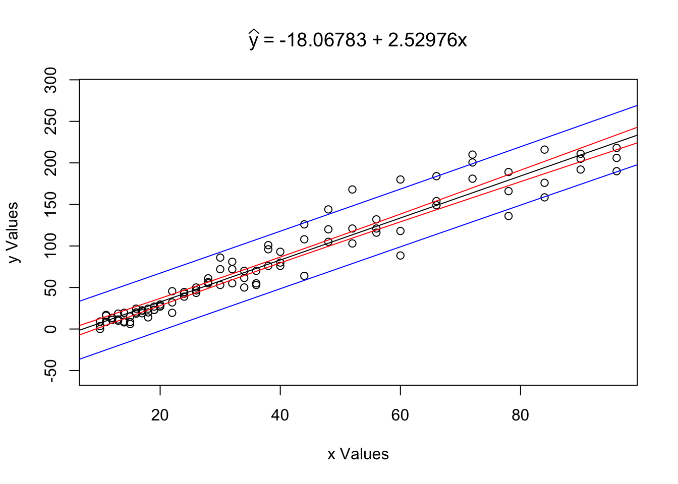
Figure 12.5: Regression Analysis for ToyCars

What we see is the scatterplot of x = ToyCars$Height vs y = ToyCars$Distance along with super imposed blue and red lines. If we restrict our view to only values of \(y\) such that \(x\) is some fixed value (i.e. \(x_0\)) these lines form the confidence interval for the mean of \(y\), in red, as well as the prediction interval for individual values of \(y\), in blue.

To make this more clear, we can also pass RegressionInference a specific value of conf.level as well as a value of \(x_0\) (or x0 in R code) to see what it does.

RegressionInference( x = ToyCars$Height, y = ToyCars$Distance, 
                   conf.level = 0.99, x0 = 46 )

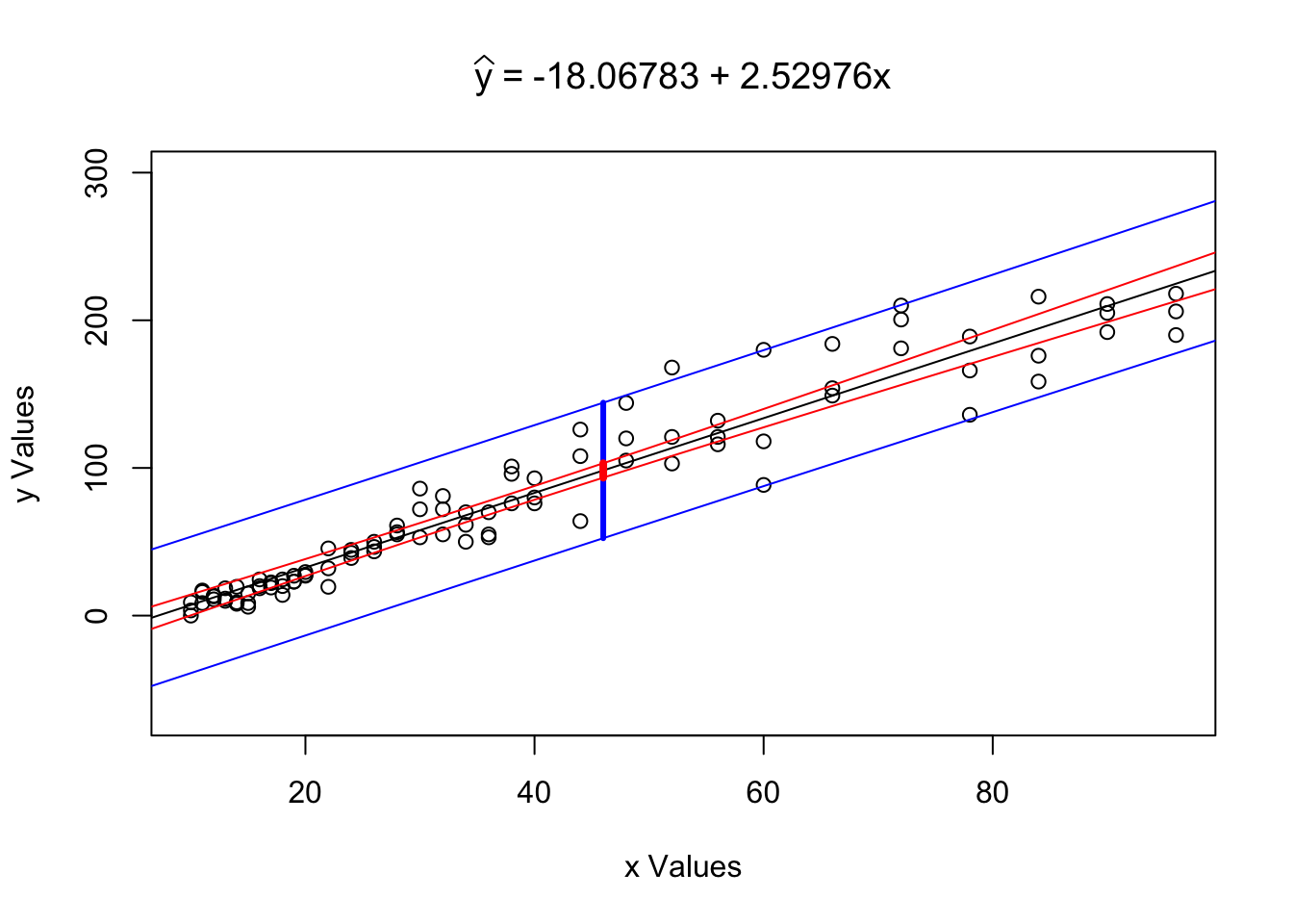
Figure 12.6: Regression Analysis for ToyCars

## $`Confidence Level`
## [1] 0.99
## 
## $`Conf. Int. for yHat`
## [1]  93.41713 103.18515
## 
## $`Pred. Int. for y`
## [1]  52.42209 144.18019
## 
## $`Tested Point`
## [1] 46
## 
## $`yHat at x0`
## [1] 98.30114

We see the same graph as before, but now also see a band drawn at \(x = x_0\). Reading the output of the function, we also see that we can make the following statements:

1. The value \(\hat{y}|_{x=46} = 98.30114\) is our point estimate (or best guess) for the distance a car will travel when dropped from a height of 46 inches. This is our best guess for both the mean distance a car would travel as well as our best guess for the distance a random car would travel.

2. We are 99% confident that the mean distance a car will travel when dropped from a height of 46 inches is between 93.41713 and 103.18515 inches.

3. We predict that 99% of individual cars will travel between 52.42209 and 144.18019 inches when dropped from a height of 46 inches.

Statement 2. is the typed out version of the confidence interval for \(\mu_y|_{x=x_0}\) based on the point estimate \(\hat{y}|_{x=x_0} = 98.30114\).

Statement 3. is the interpretation of our prediction interval for individual values of form \(y|_{x=x_0}\). The prediction interval also has a point estimate of \(\hat{y}|_{x=x_0} = 98.30114\), but takes on a larger standard error as shown above.

The prediction interval for \(x=x_0\) should be interpreted as the interval between the bottom of the bottom blue segment to the top of the top blue segment and thus containing the red segment as well. The prediction interval for \(y|_{x=x_0}\) will always contain the confidence interval for \(\mu_y|_{x=x_0}\) if they are at the same confidence interval.

Use the methods shown in Example 12.6 above to make statements about a newborn’s father’s age if its mother was 38 at the time of its birth.

Remark. Like we did for LinearRegression, the function RegressionAnalysis also has an Advisable Range that is between \[\text{min}({\bf x}) - 0.05 ( \text{Max}({\bf x}) -\text{min}({\bf x}) )\] and \[\text{Max}({\bf x}) + 0.05 ( \text{Max}({\bf x}) -\text{min}({\bf x}) ).\] While these functions will allow a tiny bit of extrapolation, they are built with some internal warnings. See Example 5.15 for an example of how the advisable range works. In fact, the code in that example can be exactly replicated by simply replacing LinearRegression with RegressionInference.

Exercises

Remark. For Exercises 12.1 through 12.3, you will need to load the dataset hot_dogs. The code for this can be found in Example 1.7.

For Exercises 12.4 through 12.6, you will need to load the dataset BabyData1. The code for this can be found in Example 4.1.

For Exercises 12.7 through 12.8, you will need to load the dataset TitanicDataset. The code for this can be found in Example 10.15.

Exercise 12.1 Using the hot_dogs dataset, find a 99% confidence interval for the population correlation coefficient between a hot dog’s calories and sodium level.

Exercise 12.2 Using the hot_dogs dataset, test whether there is any true correlation between a hot dog’s calories and sodium level.

Exercise 12.3 Using the hot_dogs dataset, give both a prediction interval for individual sodium values as well as a confidence interval for the mean sodium level for a hot dog which has 150 calorie at a 97% confidence level. Explain the difference between the two intervals.

Exercise 12.4 Using the BabyData1 dataset, give a 90% confidence interval for the population correlation coefficient between the length of a baby’s gestation and its birth “weight.” Use both the rhoConfInt and cor.test to find the interval.

Exercise 12.5 Using the BabyData1 dataset, give a 97% prediction interval for the age of a newborn’s father if the mother was 25. Interpret this result.

Exercise 12.6 Using the BabyData1 dataset, give a 98% confidence interval for the mean age of a newborn’s father if the mother was 25. Interpret this result.

Exercise 12.7 Using TitanicDataset, give a 95% confidence interval for the population correlation coefficient between a passenger’s age and the fare they paid. Interpret this result.

Exercise 12.8 Using TitanicDataset, test the claim that there was correlation between a passenger’s age and the fare they paid. Interpret this result at the \(\alpha = 0.02\) level of significance.

12.3 Appendix

12.3.1 rhoConfInt

rhoConfInt <- function( x, y, conf.level = 0.95, size = 10000 ){
  xVec <- x
  yVec <- y
  OK <- complete.cases(xVec, yVec)
  x <- xVec[OK]
  y <- yVec[OK]
  if( length(x) != length(xVec) )
    warning("Missing values omitted from calculations")
  n1 <- length( x )
  CILp <- (1 - conf.level) / 2
  CIUp <- 1 - CILp
  rValues <- replicate( n = size , {
    NewOrder <- sample( x = 1:n1, replace = TRUE )
    cor( x[ NewOrder ], y[ NewOrder ] )
  })
  rHist <- hist( rValues, plot = FALSE )

  xDelta <- rHist$breaks[2] - rHist$breaks[1]
  CIL <- quantile( x = rValues, probs = CILp )
  xL <- rHist$breaks[ min(which( rHist$breaks > CIL)) ]
  yL <- rHist$counts[ min(which( rHist$breaks > CIL)) ]

  CIU <- quantile( x = rValues, probs = CIUp )
  xR <- rHist$breaks[ max(which( rHist$breaks < CIU)) ]
  yR <- rHist$counts[ max(which( rHist$breaks < CIU)) ]

  CILength <- round((xR - xL) / xDelta)

  xValues <- c( rep(
    c( CIL ,seq( from = xL, to = xR, by = xDelta ), CIU ),
    each = 2)
  )
  yValues <- c( 0,
                rep(
                  rHist$counts[ min(which( rHist$breaks > CIL)) -2 + 1:(CILength+2)],
                  each = 2),
                0)

  hist(rValues)
  polygon(xValues,yValues,col='skyblue', density = 50)

  Results <- list("Confidence Level" = conf.level, 
                 "Confidence Interval" = c( CIL, CIU ),
                 "How Many Shuffles" = size )  
  return(Results)
}

12.3.2 RegressionInference

RegressionInference <- function( x, y, conf.level = 0.95, x0 = "null" ){
  xVec <- x
  yVec <- y
  OK <- complete.cases(xVec, yVec)
  x <- xVec[OK]
  y <- yVec[OK]
  if( length(x) != length(xVec) )
    warning("Missing values omitted from calculations")
  xBar <- mean( x )
  SumSquareDevx <- sum( (x - xBar)^2)
  Residy <- residuals( lm( y ~ x ) )
  SumSquareResidy <- sum( Residy^2 )
  n <- length( y )
  SEyHat <- sqrt( SumSquareResidy / ( n - 2 ) )
  a <- (summary(lm(y~x))$coefficients[1, 1])
  b <- (summary(lm(y~x))$coefficients[2, 1])
  tStar = qt( 1 - (1 - conf.level)/2, df = n-1)
  SEyhat <- function(x0){SEyHat * sqrt( 1/n + (x0 - xBar)^2 / SumSquareDevx)}
  SEyhatPrediction <- function(x0){
    SEyHat * sqrt( 1/n + (x0 - xBar)^2 / SumSquareDevx + 1)}
  xDelta <- ( max(x) - min(x) )/100
  xMin <- min(x) - 5*xDelta
  xMax <- max(x) + 5*xDelta
  xValues <- seq( from = xMin, to = xMax, by = xDelta)

  yLower <- function(x){ a + b*x - tStar*SEyhat(x)}
  yUpper <- function(x){ a + b*x + tStar*SEyhat(x)}

  yLowerValues <- yLower(xValues)
  yUpperValues <- yUpper(xValues)

  yLowerPrediction <- function(x){ a + b*x - tStar*SEyhatPrediction(x)}
  yUpperPrediction <- function(x){ a + b*x + tStar*SEyhatPrediction(x)}

  yLowerPredictionValues <- yLowerPrediction(xValues)
  yUpperPredictionValues <- yUpperPrediction(xValues)

  yMin <- min( c( y, yLowerPredictionValues) )
  yMax <- max( c( y, yUpperPredictionValues) )
  Margin <- 0.05 * (yMax - yMin)

  plot(x,y,xlab="x Values",ylab="y Values",
       ylim = c( yMin - Margin, yMax + Margin),
       main=bquote(widehat(y)~"="~.(summary(lm(y~x))$coefficients[1, 1])~"+"
                   ~.(summary(lm(y~x))$coefficients[2, 1])*"x"))
  abline(lm(y~x))

  lines( xValues, yLowerValues, col = "red")
  lines( xValues, yUpperValues, col = "red")

  lines( xValues, yLowerPredictionValues, col = "blue")
  lines( xValues, yUpperPredictionValues, col = "blue")

  if( x0 != "null" )
    {
      if( x0 < xMin | x0 > xMax )
         warning( "Value outside of Advisable Range" )
      if( x0 >= xMin & x0 <= xMax )
          { xCord = c( x0, x0)
            yCord1 = c( yLowerPrediction(x0), yUpperPrediction(x0))
            yCord2 = c( yLower(x0), yUpper(x0) )
            lines( xCord, yCord1, col = "blue", lwd =3)
            lines( xCord, yCord2, col = "red", lwd =4)
                Results <- list( "Confidence Level" = conf.level,
                   "Conf. Int. for yHat" = yCord2,
                   "Pred. Int. for y" = yCord1,
                   "Tested Point" = x0,
                   "yHat at x0" = a + b*x0
                     )
        return(Results)}
      }
}

---

147. Fauna of Australia. Vol. 1b. Australian Biological Resources Study (ABRS)↩︎

148. Sadly, \(r\) is a biased estimator of \(\rho\), but an unbiased estimator is well beyond the scope of this book. See this Article for more.↩︎

149. As mentioned elsewhere, we have chosen to focus on Pearson’s Correlation Coefficient on Statypus, but there are alternate ways to investigate correlation. The curious reader can begin an investigation at Wikipedia.↩︎

150. This method is only given a cursory coverage here. The curious reader can see Wikipedia to begin a further exploration of this concept.↩︎

151. While there is no mathematical or statistical importance to this footnote, we would be remiss if we were to miss an opportunity to make a covert reference to one of the greatest spies of fiction, James Bond.↩︎

152. The curious (and ambitious) reader can begin by looking at this portion of a book by Dr. Darrin Speegle and Dr. Bryan Clair. The whole book can be found at https://probstatsdata.com/ and is a great place to study further than shown on Statypus if you have a calculus background.↩︎