Chapter 9 Inference for Population Proportion(s)

Figure 9.1: A Sample of Statypi

More than one platypus is (probably) called platypuses, although this is slightly debated. The term platypus is derived from Greek and platypuses follows the established convention of plural forms of Greek nouns. Ironically, the Greek plural of platypus is platypodes. There is also a healthy minority of English speakers that prefer the informal term platypi.⁸⁷

We are often interested in knowing what proportion of a population has a certain trait. That trait may be planning to vote yes on a certain proposition, a particular blood type, M&Ms that are blue, girls in different populations, or choosing to exercise at least three times per week. It is often unfeasible, if not impossible, to know parameters for a variety of reasons. Regardless, we want to know as much about the value of parameters as we can and this is the main goal of Inferential Statistics, that is inferring information about a population from the values of statistics from a sample.

For example, if you want to know if a certain proposition will be approved by voters in an upcoming election, we would need to know the population proportion for this trait. However, due to numerous factors, not the least of which is the fact that some people do not make up their mind until the actual moment they cast their vote, it is impossible to know this value in advance. So, we are forced to take a sample of the voters, and use this proportion to give our best guess as to whether the actual proportion of voters will allow for the proposition to pass.

New R Functions Used

All functions listed below have a help file built into RStudio. Most of these functions have options which are not fully covered or not mentioned in this chapter. To access more information about other functionality and uses for these functions, use the ? command. E.g. To see the help file for qnorm, you can run ?binom.test or ?binom.test() in either an R Script or in your Console.

binom.test(): This function can be used for testing that the proportions (probabilities of success) in one or several groups are the same, or that they equal certain given values.

9.1 Part 1: Distribution of Sample Proportions

Suppose we are working with a university whose population is 60% female with 6000 females and 4000 people who do not identify as female. The population can be viewed by a bar plot as below.⁸⁸

Figure 9.2: Bar Plot of University Genders

This is one population of individuals where each individual is an actual person at the university.

We now want to consider a different population that is created by sampling the above population. The histogram says that we expect 30 out of every 50 students to identify as female. However, it is fairly obvious that if we took repeated different samples of size 50 from the university population that we wouldn’t always get 30 females. (Samples are allowed to share individuals from the university.) So, we now consider what sort of distribution the proportion of females from each sample would give. We expect that we would get that the proportion would be $0.6 = \frac{30}{50}$, but it would not be shocking to get values such as $0.58 = \frac{29}{50}$ or $0.64 = \frac{32}{50}$. However, it would be fairly unlikely to get a sample which has a proportion less than $\frac{1}{3}$. In fact, we will show that the probability of choosing a sample having a proportion of females less than $\frac{1}{3}$ is less than six tenths of one percent of one percent, that is approximately 0.00006.⁸⁹

9.1.1 Formal Setup

Definition 9.1 If we consider a population of size $N$⁹⁰ where a proportion of individuals have a certain trait, this is a parameter known as the population proportion and is denoted as $p$.

Actually attaining the value of $p$ is often difficult, if not impossible, as it would likely require a census of the entire population. We can get an estimate of this parameter by taking a sample and getting a statistic from it.

Definition 9.2 If we take a sample of size $n$ and count the number of individuals, which we will call $x$, which have the desired trait, then we can define the sample proportion to be

\[\hat{p} = \frac{x}{n}.\]

The sample proportion $\hat{p}$ is the point estimate of the population proportion as it is our best guess for $p$ given a single sample, but it is only a single point with no margin of error. This is a concept we will further investigate in this chapter.

Remark. Some readers may be wondering about why we choose to use $p$ when Greek letters have been our mainstay for parameters. There is a Greek letter that is often used for the population proportion, but it is $\pi$. It was decided that the pattern of the use of Greek letters for parameters was not as important as avoiding the almost certain confusion between $\pi$ being the population proportion (and thus necessarily between 0 and 1) and the constant ratio of a circle’s diameter to its radius ($\approx 3.14159$).

In addition, there is a parameter that we did not introduce in Chapter 5. We defined $r$ to be the correlation coefficient between two sets of data. However, more formally, $r$ is the sample correlation coefficient, and thus a statistic. $r$ is a point estimate of the population correlation coefficient which is traditionally denoted by the Greek letter $\rho$, pronounced the same as “row.” That is \[r \approx \rho.\] This is explored in Chapter 12 when we do inferential statistics on the least squares regression line.

9.1.2 Notation

Definition 9.3 We summarize the notation we have at this point.

Parameter: A value that describes a characteristic of a population.
Census: A device used to gather information from an entire population.
$N$: The population size. [Note: May be infinite.]
$p$: The population proportion.
Statistic: A values taken from a sample.
Survey: A device used to gather information from a sample.
$n$: The sample size.
$x$: The number of individuals in a sample with the desired trait.
$\hat{p}$: The sample proportion, our point estimate of $p$.
Point estimate: A single value derived from statistics used to estimate a parameter.

Example 9.1 Suppose we want to find the proportion of M&M candies that are primary colored. That is, what proportion, $p$, of M&Ms are Red, Yellow, or Blue. We can consider the population to have $N = \infty$ as hundreds of millions of M&Ms are made every single day and the rate has been growing each year. If you were to be handed a Fun Size bag of Milk Chocolate M&M Candies by your professor and the bag contained 16 total candies of which 7 are primary colored, then we would get that

\[\hat{p} = \frac{7}{16} = 43.75\%\] This value is our point estimate of $p$ and would be our best guess if we had to pick a single value. It seems clear that the probability that $p$ is EXACTLY $\frac{7}{16}$ is likely very small, if not 0, so we will need to include the concept of a Margin Of Error to have any chance of making a true inference (guess) about $p$. We will do this in Section 9.2 and we will return to this example as we develop more tools.

9.1.3 Set Up and Theory

To understand how close our point estimate, $\hat{p}$, is to being the parameter, $p$, we must first understand the population of all possible cases of $\hat{p}$. That is, we will now consider a population where individuals are values of $\hat{p}$. That is we consider all possible different samples of the population and take the value of $\hat{p}$ from each sample to be the individuals of a new population.

It only makes sense to compare samples of the same size, so we will assume that all samples are of an arbitrary size of $n$.⁹¹ If we look at any one individual in the sample, there is a probability of $p$ that that individual the particular trait we are interested in. To simplify linguistics and draw a connection, we will say that an individual that has the particular trait is a “success” and one that does not have the trait is a “failure.” That is, there is a probability of $p$ that the first individual is a “success.” If $n$ is significantly less than $N$,⁹² then the selection of each subsequent individual will still result in a probability of $p$ of finding a “success.”⁹³ That is, we have $n$ independent individuals who each result in either a “success” or “failure.” We illustrate this with a little “example.”

Example 9.2 Suppose there is a party and there are 4 cupcakes on a table, 2 of which are chocolate and the other 2 are strawberry. If you were to be given a cupcake at random, it is clear that $P(\text{Chocolate}) = \frac{1}{2}$. But, what if you weren’t the first person to receive a cupcake? Whichever type of cupcake that is given out first will greatly impact your chances of receiving a chocolate cupcake. We would get the following probabilities.

\[\begin{align*} \text{First Cupcake is Chocolate} &\rightarrow P(\text{Chocolate}) = \frac{1}{3} \approx 33.33\%\\ \text{First Cupcake is Strawberry} &\rightarrow P(\text{Chocolate}) = \frac{2}{3} \approx 66.67\% \end{align*}\]

However, now imagine you are at a factory where there are many cupcakes of each variety. Let’s say, for discussion purposes, that there are 1,000 of each type, chocolate and strawberry.. If you get the first cupcake, we get that $P(\text{Chocolate}) = \frac{1000}{2000} = \frac{1}{2}$. However, if we get the second cupcake, we get the following probabilities:

\[\begin{align*} \text{First Cupcake is Chocolate} &\rightarrow P(\text{Chocolate}) = \frac{999}{1999} \approx 49.975\%\\ \text{First Cupcake is Strawberry} &\rightarrow P(\text{Chocolate}) = \frac{1000}{1999} \approx 50.025\% \end{align*}\] Thus, the probabilities have technically changed, the change is very minimal. The probability of getting a chocolate cupcake (at random) has changed in roughly 1 part in 4000 if we get the second cupcake handed out rather than the first.

The difference between the scenarios in the above example is clear. When we sampled 2 cupcakes out of 4, the selection of the first cupcake dramatically impacted the probability of the second cupcake. However, when we sampled 2 cupcakes out of 2000, the probabilities were unchanged up to 3 digits! This leads to the following definition.

Definition 9.4 When $n$ is significantly small enough compared to $N$, so that the individuals can be viewed as independent, we will write $n << N$. This is always true when $N = \infty$ and we will take $n << N$ to mean that $\frac{n}{N} < 0.05$ to avoid the need for any finite population correction.

That is, we will write $n << N$ whenever the sample size, $n$, is less than five percent of the population size, $N$.

Remark. The choice of 5% in the above definition is a bit arbitrary. This seems to be fairly standard in the literature, but in essence, some sort of finite population correction is necessary whenever $N$ is finite. However, we will adopt this convention to allow us to utilize simpler techniques at the beginning of our statistical journey.

If we only sample a small portion of a population, we can assume that each choice is independent. Sampling a large portion of a population is possible, but requires more care and other concepts not explained here on Statypus.

One key tool we will use to understand the distribution of sample proportions is a theorem called the Central Limit Theorem. There are different versions of this theorem, but the version of interest to us is given below.

Theorem 9.1 (Central Limit Theorem (CLT)) Given a distribution or random variable, $X$, with a population mean of $\mu_X$ and a population standard deviation of $\sigma_X$, then the collection of samples of size $n$ gives rise to a distribution of sample means, $\bar{x}$, which have mean and standard deviation given below. \[\begin{align*} \mu_{\bar{x}} & = \mu_X\\ \sigma_{\bar{x}} & = \frac{\sigma_X}{\sqrt{n}} \end{align*}\]

If the original distribution was Normal, then the distribution of sample means is also Normal.
However, the distribution approaches Norm$(\mu_{\bar{x}}, \sigma_{\bar{x}})$ as $n$ gets large regardless of the shape of the original distribution.

A fun classroom demonstration of the Central Limit Theorem involves using M&M candies. The teacher instructions can be found here, the required Google sheet can be found here, and an R script to handle the random numbers involved can be found here.

Thus, in order to find $\mu_p$ and $\sigma_p$, we simply need to realize $p$ as the average of a distribution we can work with. This isn’t too hard. We let $X$ be a discrete random variable such that $P( X = 1 ) = p$ for some $p>0$ and also require $P ( X = 0 ) = 1-p$ so that the sample space of $X$ is $\{ 0,1 \}$. If we consider $X=1$ to be a success, we get that an average of a sample of $n$ values from $X$ is exactly a value of $\hat{p}$ we are after. We verify this with a short little example.

Example 9.3 We consider a coin and imagine flipping it 6 times. We can simulate this using the following code.

sample( x = c("Heads", "Tails"), size = 6, replace = TRUE )

## [1] "Tails" "Tails" "Tails" "Tails" "Heads" "Heads"

If we consider the result of “Heads” to be a success, we get that $\hat{p} = \frac{2}{6}$ or $\frac{1}{3}$. If we assign the results of the statistical experiment as below:

\[\begin{align*} \text{Heads} &\rightarrow 1\\ \text{Tails} &\rightarrow 0 \end{align*}\]

Then we get that our sample is equivalent to the vector ${\bf x} = ( 0, 0, 0,0,1,1)$ which immediately gives that $\bar{x} = \frac{1}{3}$ as well. Thus, $\bar{x} = \hat{p}$ as claimed.

Thus, we just need to find $\mu_X$ and $\sigma_X$ for a generic value of $p$ and invoke the Central Limit Theorem. Using Definition 6.5, we can do this pretty easily and we summarize the results in the following theorem.

Theorem 9.2 Given a discrete random variable such that $P( X = 1 ) = p>0$ and $P ( X = 0 ) = 1-p$, we get that

\[\mu_X = p\] and \[\sigma_X = \sqrt{p \cdot (1-p)}.\]

The proof of Theorem 9.2 can be found in this chapters appendix, Section 9.7.2.1.

The requirement that $n << N$ will allow us to pull actual samples (without replacement) from a population without affecting the “new” probability of “success” after some individuals are removed. In addition, we will require that we can expect at least 5 successes and 5 failures or that both $n \cdot p$ and $n \cdot (1-p)$ are both at least 5 so that $n$ is large enough to assume the distribution of $\bar{x} = \hat{p}$ is approximately Normal.⁹⁴

Theorem 9.3 The distribution of sample proportions, that is the collection of all possible values of $\hat{p}$ from samples of size $n$, from a population with a population proportion of $p$ is approximately Normal with the following parameters.

\[\begin{align*} \mu_{\hat{p}} & = p\\ \sigma_{\hat{p}} & = \sqrt{ \frac{ p \cdot (1-p)}{n} } \end{align*}\]

assuming that $n\cdot p \geq 5$, $n \cdot (1-p) \geq 5$, and that $n << N$.

The following exploration shows the relationship between random samples drawn with the given population proportion and sample size and the theoretical model shown above.

We begin by noting that if we alter the population proportion with the purple slider without changing the sample size that the background changes to a red color and a warning appears indicating that we have violated the conditions of Theorem 9.3. Feel free to toggle the “Normal Model” slider and see if you agree that we shouldn’t trust the model when the conditions are not met. Setting $p$ to an extreme value near 0 or 1 should show that the model does break down.

Set the sample size to 40 and the population proportion to a value around 0.7. Toggle the “Normal Model” slider to “Yes” and you should see that the histogram of random samples appears to fit the model predicted by Theorem 9.3. If you reduce the number of samples using the black vertical “# of Samples” slider on the right hand side, you should see that the agreement between the histogram and the model becomes weaker. Dragging the “Randomizer” slider will change the random samples that are shown in the histogram. Conversely, increasing the number of samples will increase the agreement between the histogram and the model. This illustrates the concept contained in the Law of Large Numbers, Theorem 6.1.

Further investigation can be done using these tools as well as the tools opened by toggling the “Probability” slider. However, we will not go further here. Reach out to your instructor or the author of Statypus if you have questions on what else you can do with this exploration.

9.1.4 Applications to the Distribution of Sample Proportions

Since there is no new functions being used in this section, we encourage the reader to use the code chunks in the following examples as their template code for problems of this type.

We return to the setup we had in the beginning of this section where we had a population which was 60% female. At this point, we will not assume that $N = 10000$, but comment on the requisite size of $N$ as we go along. So, we have that $p = 0.6$ and our initial population of individual people looks like the following histogram.

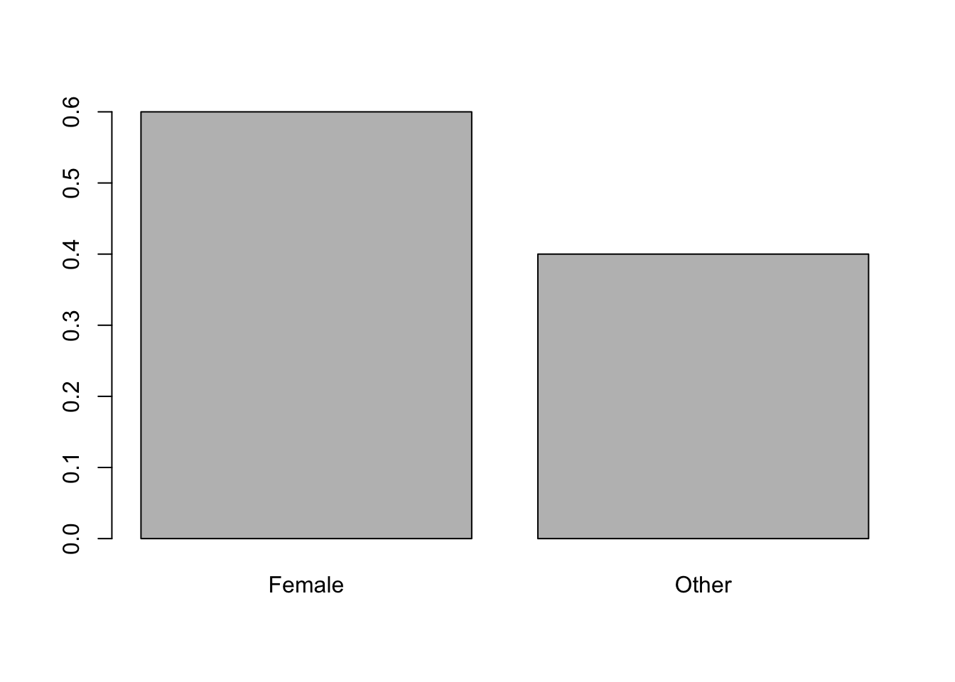
Figure 9.3: Relative Frequency Bar Plot of University Genders

Now, if we randomly select 50 people from the population, we expect to have 30 females and 20 non-females. Moreover, if the proportion of females was important to a survey we are hoping to give, then we would not want the number of females to be too far from 30.⁹⁵

Example 9.4 Q: What is the probability that a simple random sample of 50 individuals from the population discussed above would contain no more than a third of females?

We can answer this by realizing that all SRSs of size $n=50$ would meet our criteria for a Normal distribution as long as the population size is large enough. We know that $N = 10000$ so that we have that $n << N$. We can now assume that the distribution of values of $\hat{p}$ is approximately Normal with

\[\begin{align*} \mu_{\hat{p}} & = p = 0.6\\ \sigma_{\hat{p}} & = \sqrt{ \frac{ p \cdot (1-p)}{n} } = \sqrt{ \frac{ 0.6 \cdot (1- 0.6)}{100}} \approx 0.049 \end{align*}\]

We can now answer our question about an unlikely SRS having no more than a third of females with pnorm using the following code chunk.

n = 100           #Sample Size
pHat = 1/3        #Sample proportion to be tested
p = 0.6           #Population proportion
#Only change the value of `lower.tail` below and also the values above.
pnorm( q = pHat, mean = p, sd = sqrt( p * ( 1 - p ) / n ), lower.tail = TRUE )

## [1] 2.614968e-08

That is to say that we should expect a sample that under-represents females at least this much once in every 382 million (the reciprocal of the above output of pnorm) SRSs of size $n = 100$.

Example 9.5 Q: Do you think it would be more or less likely to have a smaller sample have no more than one third females?

Being that we need $n \cdot p \geq 5$ and $n \cdot (1-p) \geq 5$, we get that we need $n \geq 15$.⁹⁶ We can set the sample size to $n = 25$ to make sure the sample is not excessively small and run the above code with this new value.

n = 25            #Sample Size
pHat = 1/3        #Sample proportion to be tested
p = 0.6           #Population proportion
#Only change the value of `lower.tail` below and also the values above.
pnorm( q = pHat, mean = p, sd = sqrt( p * ( 1 - p ) / n ), lower.tail = TRUE )

## [1] 0.003247793

This says we can now expect such “unlucky” samples once in roughly every 308 SRSs of size $n = 25$. Compared to samples of size $n=100$, this is over 1 million times more likely!

Remark. This shows that $\hat{p}$ deviating a certain distance from $p$ is less likely as we increase $n$. This is exactly what the Law of Large Numbers, Theorem 6.1, told us would happen.

In Chapter 8, we discussed Steph Curry’s all time record of 91.0% free throw percentage. Let’s assume that this is the value of $p$ of the proportion of free throws that Steph Curry will make.

What is the minimal sample size, $n$, in order to believe the set of $\hat{p}$s of size $n$ is Normally distributed?
Find $\mu_{\hat{p}}$ and $\sigma_{\hat{p}}$ for samples of size $n=100$ of Steph Curry free throws.
If we use the values found in question 2 above and assume we can treat the distribution of $\hat{p}$ values are Normally distributed, redo Exercise 8.2 part c. That is, find $P( \hat{p} > 0.95)$.

Example 9.6 (Melody Returns) We can use our new tool to re-analyze the saga of Melody’s shoes which was introduced in Section 8.4. We use the same code as above and use $p = 0.5$ to assume that, at worst, we expect Melody to have a random chance of success equal to that of a Blind Ape in a Dark Room (BADR). We find the probability that a random sample of size $n = 40$ would give a value of $\hat{p}$ no higher than the observed value of $\frac{13}{40}$.

n = 40            #Sample Size
pHat = 13 / 40    #Sample proportion to be tested
p = 0.5           #Population proportion
#Only change the value of `lower.tail` below and also the values above.
pnorm( q = pHat, mean = p, sd = sqrt( p * ( 1 - p ) / n ), lower.tail = TRUE )

## [1] 0.01342835

This says that we expect a BADR to achieve a sample proportion no better than Melody only 1.34% of the time. This value is less than the one found in Section 8.4, but is very comparable. The main discrepancy is the use of the CLT as compared to using Binomial tools directly. We will see this type of discrepancy later when we use the function binom.test in Section 9.5.

9.2 Part 2: Confidence Intervals for Population Proportion

We know that the sample proportion, $\hat{p}$, is our point estimate of the population proportion, $p$. However, being that for any given value of the sample size, $n$, there are only $n+1$ possible values of $\hat{p}$, and that $p$ can be any of the infinite values between 0 and 1, we are quite certain that the probability that a given sample gives the exact value of $p$ is very small (typically 0).

9.2.1 Confidence vs. Margin of Error vs. Precision

There is a sort of tug of war between the desire for a esitmation to be precise and our confidence in that precision. In a perfect world, it would be ideal to both be extremely confident about an estimate and have a very precise estimate, however, this is not possible.

Figure 9.4: The Bullseye of a Dartboard, Photo by Martin Vorel: https://libreshot.com/

Example 9.7 To illuminate this idea, let’s consider a simple carnival game of trying to hit a bullseye with a dart from a certain distance. There seems to be a give and take between the precision of the shot needed and the confidence of the thrower. If we think of the radius of the bullseye as the margin or error granted the thrower, then it is clear that as we increase the margin of error, i.e. a larger target, that the confidence of the thrower should increase.

To make this more explicit, imagine you are standing at a standard dart board from any length. The inner or double bullseye has a radius, or margin of error, of only 0.25 inches. Try to mentally guess your probability of hitting this small target if you were given three attempts. Would you be willing to wager $1 that you could do it?

Now imagine that the game is simply whether you can hit the scoring region of the dartboard as a whole from the same distance as with the double bullseye. This has a radius, or margin of error, of just under 9 inches. Would you be willing to make the $1 wager now?

Regardless of your confidence at hitting the double bullseye, it should be true that you had more confidence at hitting the scoring region of the board. You still may not want to take the bet, but you should have had more confidence in hitting the larger target.

This example showed that as we increased the margin of error, we also increased the confidence in hitting that target. The reverse is also true, the only way to increase the confidence of a given thrower is to increase the margin of error. We write this symbolically below.

\[(\text{Confidence} \uparrow) \Leftrightarrow (\text{Margin of Error} \uparrow)\] Remembering that the target we are interested in is $p$, we can see that the margin of error is actually a measure of how precise the estimate is, but it is clear that a large margin of error would mean a low level of precision. That is, we have the following.

\[ (\text{Margin of Error} \uparrow)\Leftrightarrow (\text{Precision} \downarrow)\] Putting this together, we get the following.

For any given sample size, we get that \[(\text{Confidence} \uparrow) \Leftrightarrow (\text{Margin of Error} \uparrow) \Leftrightarrow (\text{Precision} \downarrow)\]

or logically equivalently that

\[(\text{Confidence} \downarrow) \Leftrightarrow (\text{Margin of Error} \downarrow) \Leftrightarrow (\text{Precision} \uparrow).\]

The last part says that if we want higher precision, we must have a smaller margin of error which would lower our confidence.

This exploration offers an interactive alternative to the darts thought example described above.

Begin by adjusting the green slider to a random spot to produce a random location within the white region. This becomes our target.
Memorize where the green dot is in the white field and toggle the black slider to “Guess” to hide the target and show the draggable red guess point.
Drag the red dot to the location you believe the green dot was prior to toggling the black slider.

How confident are you that the green dot is exactly aligned with the red dot? In other words, how often do you think you would win if you wagered $1 that the green dot is exactly aligned with the red dot?

Raise the vertical red slider slightly and notice that a radius is added to the red dot offering a margin of error for our guess.

How confident are you that the green dot is within the shaded red region? It should be higher than it was before because we now have a margin of error.

Adjust the vertical red slider and consider how your confidence is impacted by the size of the margin of error.

You should feel more confident with a higher margin of error and less confident with a smaller margin of error. This gives another way of seeing the relationship we stated in the Big Idea above. The only neglected aspect within this exploration is the realization that precision is inversely related to the margin of error. A more precise guess means a smaller margin of error and a less precision means we are allowed a larger margin of error.

9.2.2 Confidence Interval Code

Remark. From here on, we will denote the value of $\hat{p}$ from a sample we are actually working with as $\hat{p}_0$ (or pHat0 in R code) to distinguish it from the distribution of other possible values of $\hat{p}$.

Our goal is to give a confidence interval for the population proportion $p$. Our point estimate, $\hat{p}_0$, is an unbiased estimator⁹⁷, so we want an interval with bounds given by

\[\text{point estimate} \pm \text{Margin Of Error}\] or using the fact that we know $\hat{p}_0$ is our point estimate, we get

\[\hat{p}_0 \pm \text{Margin Of Error}\]

This just leaves us to find a formula for the Margin Of Error, which we will abbreviate as $\text{MOE}$.

Let’s pretend that we are working with an initial population that has a proportion of $p = 0.6.$ We will call this p0 in the code to align with the notation used in Section 9.3 dealing with hypothesis testing.

The code chunk before defines the characteristics of the sample we wish to examine. We treat p0 as a “secret” where we tell R the value, but we will not use it in the derivation of the confidence interval.

p0 = 0.6                         #Known population proportion (a "secret")
n = 100                          #Sample size
C.Level = 0.95                   #Confidence Level

We can now use rbinom⁹⁸ to generate a random number of successes pulled from a population where ${p = 0.6.}$ This is the only time we actually use the value of p0 = 0.6 and hereafter we will treat it as an unknown until we come to the point where we check if $p$ is indeed within our confidence interval.

x <- rbinom(1,n,p0)              #random binomial sample with given parameters
x

## [1] 54

Thus, for the discussion of this example, we will be working with a sample that had 54 successes out of 100. From this, we can begin working on developing confidence intervals. We first calculate $\hat{p}_0$ (our observed value of $\hat{p}$), denoted pHat0 here.

pHat0 <- x / n                    #Sample proportion of success
pHat0

## [1] 0.54

We would like to be able to calculate the standard deviation of the sample proportions, $\sigma_\hat{p}$, but this is likely impossible. Instead, we introduce the concept of the Standard Error attributed to a sample.

Definition 9.5 Given a sample with a sample proportion of $\hat{p}_0$ from a population being measured for a certain trait, we say that the Standard Error of The Distribution of Sample Proportions or simply the Standard Error attributed to the sample proportion $\hat{p}_0$ is the value

\[\text{SE} = \sqrt{\frac{\hat{p}_0\cdot( 1-\hat{p}_0)}{n}}\] which is an approximation to the (likely) unknown value of

\[\sigma_\hat{p} = \sqrt{\frac{ p \cdot( 1-p)}{n}}.\] We will treat the standard error like a standard deviation because it is a point estimate of one.

Remark. A lot of sources define what we have labeled $\sigma_\hat{p}$ to be the standard error and then treat the value of $\text{SE}$ as just an approximation to that. While there is nothing wrong with this viewpoint, here at Statypus we will call the value

\[\sigma_\hat{p} = \sqrt{\frac{ p \cdot( 1-p)}{n}}.\] the Standard Deviation of The Distribution of Sample Proportions and view it as a parameter where as we will call the value

\[\text{SE} = \sqrt{\frac{\hat{p}_0\cdot( 1-\hat{p}_0)}{n}}\] the Standard Error of The Distribution of Sample Proportions and view it as a parameter.

That is to say we will use the approximation

\[\text{SE} \approx \sigma_{\hat{p}}\] and maintain the convention of using Latin letters ($\text{SE}$ in this case) to be the estimates of Greek letters ($\sigma_{\hat{p}}$ in this case). At this point, we have the following pairs of statistics and parameters:

\[\begin{align*} \textbf{S}\text{ample} &\approx \textbf{P}\text{opulation}\\ \textbf{S}\text{tatistic} &\approx \textbf{P}\text{arameter}\\ \textbf{S}\text{ort of } &\approx \textbf{P}\text{erfect}\\ \bar{x} &\approx \mu\\ s &\approx \sigma\\ \text{SE} &\approx \sigma_{\hat{p}} \end{align*}\]

We can now calculate the standard error based on our samples value of $\hat{p}_0$.

SE <- sqrt(pHat0*(1-pHat0)/n)      #Approximation of Standard Error
SE

## [1] 0.04983974

We know that 95% of values of $\hat{p}$ lie within roughly 2 standard deviations (or standard errors in this case) from $p$. That is equivalent to saying that 95% of samples will give a $\hat{p}$ that is within approximately 2 standard errors of $p$. That is, if we set

\[\text{MOE} \approx 2 \cdot \text{Standard Error}\] we are on the right track. This leads us to define a Confidence Level in general.

Definition 9.6 When discussing a confidence interval, the Confidence Level is a value between 0 and 1 that states how often the procedure used will give an interval that captures the parameter. I.e. how often the parameter falls between the values which define the confidence interval.

If we are discussing a 95% Confidence Interval, then we expect the procedure used will “work” for 95 samples out of 100, on average. That is to say we are making a claim of confidence about how often a sample will give a confidence interval that works and not about the individual confidence interval given from a specific sample.

We know the value of 2 above was just an approximation based on the Empirical rule. A better value can be found from qnorm.

Definition 9.7 Given a confidence level of $C$, we define the Critical $z$-Value, which we denote $z^*$ (which we assume to be positive), to be the value such that

\[P ( - z^* < z \leq z^*)=C.\] We may talk of either $z^*$ or the pair $\pm z^*$ as being the critical $z$-value(s).

The below calculates the critical $z$-values that give the middle 95% of a distribution where there is 2.5% of values in either “wing” of the distribution.⁹⁹

#Critical z-score for this confidence level
zStar <- qnorm( 1 - (1 - C.Level) / 2 )   
zStar

## [1] 1.959964

Note that we set C.Level to be 0.95 earlier and this output is the more precise version of “2.” We call this value $z^*$ or zStar in R coding. The Margin Of Error, which we abbreviated $\text{MOE}$, is the product of $z^*$ and the standard deviation of $\hat{p}$, or

\[\text{MOE} = z^* \cdot \sigma_\hat{p}.\]

However, as we are unable to know $\sigma_\hat{p}$ without knowing $p$, we are forced to use our approximation of $\sigma_\hat{p}$, the Standard Error. That is, we have the following.

Definition 9.8 We define the Margin of Error for a Confidence Interval for a Population Proportion to be given by \[\text{MOE} = z^* \cdot \sigma_\hat{p},\] but in practice we are forced to accept the approximation of \[\text{MOE} \approx z^* \cdot \text{SE}.\]

We can now write the confidence interval as

\[\left(\hat{p}_0 \pm \text{MOE}\right) \approx \left( \hat{p}_0 \pm z^* \cdot \text{SE} \right) = \left(\hat{p}_0 \pm z^* \cdot \sqrt{\frac{\hat{p}_0\cdot( 1-\hat{p}_0)}{n}}\right).\]

Remark. This says that we expect that 95% of all samples pulled from a population with a proportion of p would create a confidence interval, using the above formula, that would contain p.

Using the calculations above, we can find these bounds with the following code.

CIL <- pHat0 - zStar*SE         #Confidence Interval Lower Bound
CIU <- pHat0 + zStar*SE         #Confidence Interval Upper Bound
c( CIL, CIU )                   #Confidence Interval

## [1] 0.4423159 0.6376841

This gives a 95% confidence interval of

\[ \left(\hat{p}_0 \pm z^*\cdot SE\right) = \left( 0.54 \pm 1.959964 \cdot 0.04983974 \right) = \left( 0.44232, 0.63768\right).\] Thus, our sample did give a confidence interval that contains $p$ =p0 = 0.6. To be precise about what we mean about our confidence, 95% of all random samples will give a confidence interval that captures $p$. So, if we view our sample as one random sample pulled from all possible samples, then we have a 95% chance that our sample does give a confidence interval that contains $p$ and we indeed get that $0.4423481 <p < 0.8376519$.

Theorem 9.4 Here we summarize our results and calculations for the confidence interval for a population proportion. If $n \cdot \hat{p} > 5$, $n \cdot ( 1 - \hat{p}) >5$, and $n << N$, then we can find a confidence interval as shown below.

\[\begin{align*} \text{Conf. Int.} &= \left(\text{Pt. Est.} \pm MOE\right)\\ &= \left( \hat{p}_0 \pm z^* \cdot SE \right)\\ & = \left(\hat{p}_0 \pm z^* \cdot \sqrt{\frac{\hat{p}_0(1-\hat{p}_0)}{n}}\right) \end{align*}\]

where

\[\begin{align*} \text{Pt. Est.} & = \text{A point estimate of the parameter.}\\ \hat{p} &= \text{Sample Proportion of Success}\\ \hat{p}_0 &= \text{Observed value of }\hat{p} = \frac{x}{n}\\ x &= \text{Number of Successes}\\ n &= \text{Sample Size}\\ N &= \text{Population Size}\\ MOE &= \text{Margin Of Error} = z^* \cdot SE\\ \text{C.Level} &= \text{Desired Confidence Level}\\ z^* & = \text{zStar} = \text{qnorm( 1 - (1 - C.Level) / 2 )}\\ SE &= \text{Standard Error} = \sqrt{\frac{\hat{p}_0 \cdot (1-\hat{p}_0)}{n}}. \end{align*}\]

The code to make all of these calculations is contained in the Code Template below.

x =                 #Number of "Good" cases: User must supply this value.
n =                 #Sample Size: User must supply this value.
C.Level =           #Confidence Level: User must supply this value.
#Only change values above this line
pHat0 <- x / n      #Sample proportion
SE <- sqrt( pHat0 * (1 - pHat0) / n )
zStar <- qnorm( 1 - (1 - C.Level) / 2 )
MOE <- zStar * SE
CIL <- pHat0 - MOE  #Confidence Interval Lower Bound
CIU <- pHat0 + MOE  #Confidence Interval Upper Bound
c( CIL, CIU )       #Confidence Interval

Example 9.8 We can return to the setup in Example 9.1 and find a confidence interval for the population proportion of primary colored Milk Chocolate M&M Candies, $p$. We had 7 primary colored M&M candies out of 16 in our Fun Size bag which served as our sample. We can input these numbers into our above code and construct a 95% confidence interval for $p$.

x = 7               #Number of "Good" cases
n = 16              #Sample Size
C.Level = 0.95      #Confidence Level
#Only change values above this line
pHat0 <- x / n      #Sample proportion
SE <- sqrt( pHat0 * (1 - pHat0) / n )
zStar <- qnorm( 1 - (1 - C.Level) / 2 )
MOE <- zStar * SE
CIL <- pHat0 - MOE  #Confidence Interval Lower Bound
CIU <- pHat0 + MOE  #Confidence Interval Upper Bound
c( CIL, CIU )       #Confidence Interval

## [1] 0.1944261 0.6805739

This means that we are 95% confident that between 19.4% and 68.1% of Milk Chocolate M&M candies are primary colored. This is a very wide interval (high margin of error or small level of precision), but that is easily explained by our very small sample size of $n=16$.

9.2.3 Sample Size for Desired Confidence

We can also consider how sample size affects confidence intervals. Returning to our carnival game analogy (Example 9.7), it seems clear that your confidence would be lower if you were given only a single dart versus the ability to throw multiple darts. Moreover, the more darts that you are allowed to throw, your chance of winning definitely increases if you only need to have one dart hit the given region. Sample size plays the same roll as the number of darts we are allowed to throw. This means we have the following relationships where we imagine the Margin of Error (and thus the precision) as being fixed at one particular level, i.e. either the bullseye or the entire scoring region.

We can fix the Margin of Error (and thus the Precision) and get that the sample size moves in the same direction as the confidence. That is, we get that

\[(\text{Sample Size} \uparrow) \Leftrightarrow (\text{Confidence} \uparrow)\] and

\[(\text{Sample Size} \downarrow) \Leftrightarrow (\text{Confidence} \downarrow).\]

Remark. The above Big Idea means that we can adjust our sample size to get a desired confidence level for a desired margin of error. That is to say, if we want to know a population proportion to within five percentage points, for example, then we can do that for any selected confidence level as long as we are able to get a sample size which is sufficiently large.

To see if our intuition about the relationship between sample size and confidence is correct, we will find the sample size needed for a certain confidence level and margin of error. To do this we begin with the equation for the margin of error and solve for the value of $n$.

\[\begin{align*} \text{MOE} &= z^* \sqrt{ \frac{ \hat{p}_0 \cdot (1- \hat{p}_0)}{n}}\\ \text{MOE}^2 &= \left( z^* \right)^2 \cdot \frac{ \hat{p}_0 \cdot (1- \hat{p}_0)}{n}\\ n &= \left( z^* \right)^2 \frac{ \hat{p}_0 \cdot (1- \hat{p}_0)}{\text{MOE}^2} \end{align*}\]

Remark. If you have a prior estimate $\hat{p}_0$ of $p$, you can try the formula above to find the minimum sample size, $n$. However, it should be made clear that any inaccuracy in $\hat{p}_0$ could cause $n$ to be too low for the desired margin of error. We need to dive a bit deeper to ensure that $n$ is indeed large enough regardless of prior knowledge (or lack thereof).

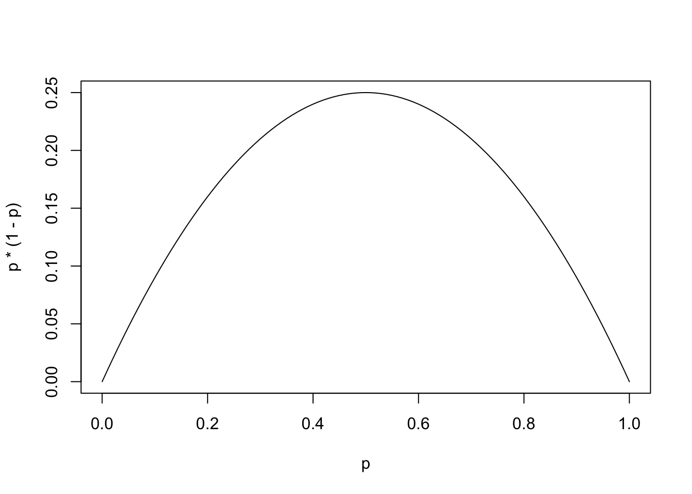
Being that we are trying to find the required sample size for a sample to calculate $\hat{p}_0$, it is possible that we have no prior value of $\hat{p}_0$ and thus need to understand how the term $\hat{p}_0 (1 - \hat{p}_0)$ affects the formula we have for $n$. We recall that Exercise 1.4 from Chapter 1 asked us to plot the curve $f(p) = p \left( 1-p\right)$ for $p \in [0,1]$. The range of this function are precisely the values that the term $\hat{p}_0 (1 - \hat{p}_0)$ can take.

Figure 9.5: Plot of f(p) = p(1-p)

As this is the graph of $f(p) = p (1-p) = p - p^2$ we see that it is a parabola and we know that the maximum value occurs midway between the two zeros of $p = 0, 1$. Therefore, the function takes on a maximum value at $p = \frac{1}{2}$ where $f\left( \frac{1}{2} \right) = \frac{1}{4}$. This proves that for any statistic, $\hat{p}_0$. we get that

\[\hat{p}_0 \cdot (1- \hat{p}_0) \leq \frac{1}{4}.\]

This now gives us that \[n = \left( z^* \right)^2 \frac{ \hat{p}_0 \cdot (1- \hat{p}_0)}{\text{MOE}^2} \leq \frac{ \left( z^* \right)^2}{4 \cdot \text{MOE}^2}.\]

Theorem 9.5 To obtain a confidence interval for a population proportion with a margin of error now larger than $\text{MOE}$ at a confidence level of $\text{C.Level}$, you should use a Minimum Sample Size of at least \[\frac{ \left( z^* \right)^2}{4 \cdot \text{MOE}^2} \geq n\] where $n$ is the theoretical minimum sample size without our removal of the $\hat{p}_0$ terms.

This code chunk gives a way to use R to calculate $n$, here denoted minSampleSize, using the above formula. We have also invoked the R function ceiling() which will round up the value of minSampleSize to give an integer value.

MOE =             #Desired Margin of Error
C.Level =         #Confidence Level
#Only change values above this line
zStar <- qnorm( 1 - (1 - C.Level) / 2 )
minSampleSize <- ceiling( zStar^2 / ( 4 * MOE^2 ) )
minSampleSize

Example 9.9 We found a confidence interval for the population proportion of primary colored M&M candies in Example 9.8. However, in that example, we found a margin of error of over 24.3% due to the exceptionally small sample size. If we wanted a confidence interval with a smaller margin of error, we would need to increase the sample size based on Theorem 9.5.

MOE = 0.1            #Desired Margin of Error
C.Level = 0.95       #Confidence Level
#Only change values above this line
zStar <- qnorm( 1 - (1 - C.Level) / 2 )
minSampleSize <- ceiling( zStar^2 / ( 4 * MOE^2 ) )
minSampleSize

## [1] 97

This says that the minimum sample size needed to achieve a margin of error of $0.1$ at the 95% confidence level is 97.

If we choose a confidence level near $95\%$, we get that $z^* \approx 2$ so that $\frac{\left(z^*\right)^2}{4} \approx 1$. More accurately, the confidence level given by pnorm( 2 ) - pnorm( -2 ) would give that $z^* = 2$ and simplify the above formula to

\[\frac{1}{\text{MOE}^2} \geq n.\] The exact confidence level for this simplification is below.

pnorm( 2 ) - pnorm( -2 )

## [1] 0.9544997

Theorem 9.6 If we want to consider confidence levels of approximately $95\%$,¹⁰⁰ then we can use the formula

\[\frac{1}{\text{MOE}^2}\]

for our minimum sample size which can be found with even a basic function calculator. We will call this the Minimum Sample Size Rule of Thumb.

Example 9.10 For example, if we revisit Example 9.9 above, we can get $n$ by simply calculating $\frac{1}{0.1^2}$ which is $\frac{1}{0.1^2} = \frac{1}{0.01} = 100$ which is very close to the value we found initially. The slightly higher value of $n$ does give us the slightly higher confidence level of $95.45\%$ compared to the $95\%$ we used in Example 9.9.

Example 9.11 To see how the margin of error affects the minimum sample size needed, we can redo Example 9.9 but change the desired margin of error to be $0.01$.

MOE = 0.01            #Desired Margin of Error
C.Level = 0.95        #Confidence Level
#Only change values above this line
zStar <- qnorm( 1 - (1 - C.Level) / 2 )
minSampleSize <- ceiling( zStar^2 / ( 4 * MOE^2 ) )
minSampleSize

## [1] 9604

This says that the minimum sample size needed to achieve a margin of error of $0.1$ at the 95% confidence level is 9604.

We can also compare this to the Minimum Sample Size Rule of Thumb.

1/MOE^2

## [1] 10000

This shows that the rule of thumb gives a value that is very consistent with the results of Theorem 9.5.

Comparing this example to Example 9.9, we see that each sample size found here is one hundred times the values found before for MOE = 0.1.

If we have a sample with a certain margin of error at a specific confidence level, to reduce the margin of error by a factor of $n$, we need a sample size that is $n^2$ times larger. For example, if we want to cut the margin of error in half, we need a sample that is four times larger.

If we wanted to gain another decimal of accuracy, we would need to cut the margin of error by a factor of ten which means we would need a sample that is one hundred times larger than the original sample.

9.2.4 Confidence Interval Applications

Example 9.12 (College Population) Early in Part 1 of this chapter, we investigated a university population that was 60% female. However, we never stopped to ask how we obtained the exact value of the parameter. Suppose we had a SRS of 50 students from a university and 32 identified as female. From this sample, what can we confidently say about $p$?

If we use the most common confidence level of 95%, we can find this confidence interval with the following code.

x = 32              #Number of "Good" cases
n = 50              #Sample Size
C.Level = 0.95      #Confidence Level
#Only change values above this line
pHat0 <- x / n      #Sample proportion
SE <- sqrt( pHat0 * (1 - pHat0) / n )
zStar <- qnorm( 1 - (1 - C.Level) / 2 )
MOE <- zStar * SE
CIL <- pHat0 - MOE  #Confidence Interval Lower Bound
CIU <- pHat0 + MOE  #Confidence Interval Upper Bound
c( CIL, CIU )       #Confidence Interval

## [1] 0.5069532 0.7730468

Remark. The above code shows the all the calculations being made individually. It is possible to make the calculations for CIL and CIU in fewer lines of code, but they would be necessarily more complicated.

Here at Statypus, we try to write code that can be understood as easily as possible and which saves parts of the calculations to your environment if they want to be looked at.

To summarize, this means from our small sample that our single best guess, or point estimate is 0.64, but we have very little confidence (likely 0%), that $p$ is exactly 0.64. However, we have 95% confidence that CIL<$p$<CIU or $0.5069532 <p < 0.7730468$ or that $p$ is approximately between 50.7% and 77.3%.

Remark. All of the values above are stored in memory and not automatically displayed to the reader other than the final output of CIL and CIU. However, to find the value of any of other terms, you only need to type the name into RStudio and execute it. For example, to find the Margin Of Error, we can simply run the line MOE.

MOE

## [1] 0.1330468

This states that for our confidence interval, the margin of error is approximately 12.6%.

We have a 95% chance that our sample will yield a “good” confidence interval (i.e. one that contains $p$) and we indeed get that $0.5069532 <p < 0.7730468$. If we want to add confidence, we know from before that we should expect the margin of error to also increase (unless we also altered the sample size, which we won’t do here). Since we are only considering our one sample, the values of $n$ and $\hat{p}_0$ will not change and therefore the value of the Standard Error,

\[SE = \sqrt{ \frac{\hat{p}_0 \cdot (1-\hat{p}_0)}{n}},\] does not change.

The value of $z^*$, however, is calculated directly from the confidence level. If we choose to set the confidence level to 99%, we can find the new value of $z^*$ using the code below.

C.Level = 0.99
zStar <- qnorm(1-(1-C.Level)/2)   #Critical z-score for this confidence level
zStar

## [1] 2.575829

That is we get that if the confidence level if 0.99, or 99%, that $z^* \approx 2.6$ versus the approximate value of 2 we had for 95% confidence. This will give a wider confidence interval than we had before. We can find the interval by the last few lines of code that followed the calculation of $z^*$ and also display MOE in this instance.

MOE <- zStar * SE
MOE
CIL <- pHat0 - MOE  #Confidence Interval Lower Bound
CIU <- pHat0 + MOE  #Confidence Interval Upper Bound
c( CIL, CIU )       #Confidence Interval

## [1] 0.1748531

## [1] 0.4651469 0.8148531

That is, we are 99% confident that $p$ is between 46.5% and 81.5% which has a margin of error of 0.1748531. This was done with a sample of size only $n=50$. We could increase our precision if we had a larger sample.

As we discussed earlier, we can increase confidence with a given sample or a sample of the same size, but the penalty is a less precise confidence interval.

Using Example 9.8 as your guide, find a 95% confidence interval for the population proportion of primary colored M&M candies if you use a sample from a standard size bag and observe 246 primary colored M&M candies out of 506 total M&M candies. How does the larger sample impact the confidence interval? What if you increase the confidence level to 98%?

Example 9.13 (What proportion of babies born in the US are girls?) According to the 2000 National Vital Statistics Report, the number of boys born in the US in 2000 was 2,076,969 and the number of girls born was 1,981,845¹⁰¹. This sample shows that $\hat{p}_0 = \frac{1981845}{1981845 + 2076969} \approx 0.4883$ which is close to the 50% that a lot of people would guess. Is it possible that the actual population proportion, $p$, is actually 0.5? Our first method for attacking this question is to find a confidence interval for $p$ given our sample.

b = 2076969
g = 1981845
x = g
n = b+g
pHat0 <- x / n      #Sample proportion
pHat0

## [1] 0.4882818

This gives us our setup and shows the approximation of $\hat{p}_0$, 0.4882818. We can now find confidence intervals with confidence levels of 0.9, 0.95, and 0.99 by using our code above.

C.Level = 0.9
SE <- sqrt( pHat0 * (1 - pHat0) / n )
zStar <- qnorm( 1 - (1 - C.Level) / 2 )
MOE <- zStar * SE
CIL <- pHat0 - MOE  #Confidence Interval Lower Bound
CIU <- pHat0 + MOE  #Confidence Interval Upper Bound
c( CIL, CIU )       #Confidence Interval

## [1] 0.4878737 0.4886899

C.Level = 0.95
SE <- sqrt( pHat0 * (1 - pHat0) / n )
zStar <- qnorm( 1 - (1 - C.Level) / 2 )
MOE <- zStar * SE
CIL <- pHat0 - MOE  #Confidence Interval Lower Bound
CIU <- pHat0 + MOE  #Confidence Interval Upper Bound
c( CIL, CIU )       #Confidence Interval

## [1] 0.4877955 0.4887681

C.Level = 0.99
SE <- sqrt( pHat0 * (1 - pHat0) / n )
zStar <- qnorm( 1 - (1 - C.Level) / 2 )
MOE <- zStar * SE
CIL <- pHat0 - MOE  #Confidence Interval Lower Bound
CIU <- pHat0 + MOE  #Confidence Interval Upper Bound
c( CIL, CIU )       #Confidence Interval

## [1] 0.4876427 0.4889209

Notice how the width of the confidence “moves with” the confidence level. That is, if we increase the confidence level, we find a wider confidence interval or equivalently an increased margin of error. Equivalently, a decrease in the confidence level corresponds to a decrease in the margin of error.

Example 9.14 (Melody's Confidence) We can return to the confident and head strong little girl, Melody, and her struggles learning which shoe was which. Using the above techniques, we can find a 95% confidence for Melody’s “underlying” success rate of $p$. That is, we are trying to estimate what the value of $p$ would be if Melody was somehow frozen in time/age and she was allowed to put her shoes on an infinite number of times.

The actual calculation of the confidence interval is simply a matter of modifying the code chunk we have been using.

x = 13              #Number of "Good" cases
n = 40              #Sample Size
C.Level = 0.95      #Confidence Level
#Only change values above this line
pHat0 <- x / n      #Sample proportion
SE <- sqrt( pHat0 * (1 - pHat0) / n )
zStar <- qnorm( 1 - (1 - C.Level) / 2 )
MOE <- zStar * SE
CIL <- pHat0 - MOE  #Confidence Interval Lower Bound
CIU <- pHat0 + MOE  #Confidence Interval Upper Bound
c( CIL, CIU )       #Confidence Interval

## [1] 0.1798518 0.4701482

This means we are 95% confident that Melody’s success “parameter” is between 0.1798518 and 0.4701482. That is, we are 95% confident that Melody would NOT succeed as often as a blind ape in a dark room!

We can increase the confidence to see if the wider interval would contain the value of $p= 0.5$ that we assigned to BADRs.

x = 13              #Number of "Good" cases
n = 40              #Sample Size
C.Level = 0.99      #Confidence Level
#Only change values above this line
pHat0 <- x / n      #Sample proportion
SE <- sqrt( pHat0 * (1 - pHat0) / n )
zStar <- qnorm( 1 - (1 - C.Level) / 2 )
MOE <- zStar * SE
CIL <- pHat0 - MOE  #Confidence Interval Lower Bound
CIU <- pHat0 + MOE  #Confidence Interval Upper Bound
c( CIL, CIU )       #Confidence Interval

## [1] 0.1342429 0.5157571

This shows that we cannot say we are 99% confident that $p$ isn’t 0.5 because $0.1342429 < 0.5< 0.5157571$! So while we were 95% confident that Melody wasn’t as accurate as a BADR, we are not 99% confident of the same fact. To be able to understand just what level of evidence we have against Melody will require the tools of Section 9.3.

Example 9.15 (The Unfair Coin) Imagine we flipped a coin 50 times and that it produced 32 heads. Using just this, what can be confidently said about the coin’s true proportion of heads, $p$. Running the code chunk we have been working with yields the following.

x = 32              #Number of "Good" cases
n = 50              #Sample Size
C.Level = 0.95      #Confidence Level
#Only change values above this line
pHat0 <- x / n      #Sample proportion
SE <- sqrt( pHat0 * (1 - pHat0) / n )
zStar <- qnorm( 1 - (1 - C.Level) / 2 )
MOE <- zStar * SE
CIL <- pHat0 - MOE  #Confidence Interval Lower Bound
CIU <- pHat0 + MOE  #Confidence Interval Upper Bound
c( CIL, CIU )       #Confidence Interval

## [1] 0.5069532 0.7730468

This says that we are 95% confident that $0.5069 < p < 0.7731$ meaning that there is 95% confidence in the fact that $p>0.5$ which would mean the coin is unfair.

However, if we switch to a 97.5% confidence interval and repeat the calculations, we get the following.

x = 32              #Number of "Good" cases
n = 50              #Sample Size
C.Level = 0.975     #Confidence Level
#Only change values above this line
pHat0 <- x / n      #Sample proportion
SE <- sqrt( pHat0 * (1 - pHat0) / n )
zStar <- qnorm( 1 - (1 - C.Level) / 2 )
MOE <- zStar * SE
CIL <- pHat0 - MOE  #Confidence Interval Lower Bound
CIU <- pHat0 + MOE  #Confidence Interval Upper Bound
c( CIL, CIU )       #Confidence Interval

## [1] 0.4878485 0.7921515

This says that we are 97.5% confident that $0.4878 < p < 0.7922$ meaning that we are NOT 97.5% confidence in the fact that $p>0.5$, i.e. the coin is unfair. This example shows that we are somewhere in between 95% and 97.5% confident that the coin is unfair, but we don’t yet have the techniques to fully understand this. The technique of a hypothesis test will allow us to determine an explicit measure of how much confidence we have in the fact that $p>0.5$.

9.3 Part 3: Hypothesis Test for Population Proportion

In Example 9.15, we flipped a coin 50 times and that it produced 32 heads. We were curious if the coin can be considered fair. That is, we wanted to know if $p = 0.5$ where $p$ is the underlying “true” probability (or proportion) of the coin returning heads. A 95% confidence interval did not contain 0.5, but a 97.5% confidence interval did include the proportion of 0.5. This leads us to believe that there is evidence that the actual population proportion is not 50%, but we are uncertain how strong this evidence is or how to interpret it.

9.3.1 The Concept of a Hypothesis Test

The method of determining if certain evidence is sufficient to “prove” a certain claim is very analogous to a criminal trial. So, to understand all of the components of this new method, let’s pretend we are prosecutors asked to investigate the coin in Example 9.15. There are many steps that must take place between investigating a claim and having proven the claim.

In order to prove a statistical claim, we will follow the same steps as in a criminal court case.

Step 1: A researcher (prosecutor) must choose to investigate a certain concept.

Step 2: After possibly a cursory investigation, the researcher must formally make a claim.

Step 3: The researcher then must gather evidence surrounding their claim.

Step 4: IF the evidence gathered supports their claim, then they can move to test the claim (have a trial).

Step 5: All calculations (proceedings) must be conducted under the strict assumption that our claim is false (the defendant is innocent).

Step 6: After all evidence has been examined (under the assumptions in Step 5), it must be decided if it can be believed that the evidence supporting the claim can be attributed to chance alone.

Outcome 1: If the evidence is not compelling enough, we must choose to stand by our assumption and decide that the claim cannot be proven despite the evidence supporting it (finding the defendant not-guilty).

Outcome 2: If the evidence is compelling enough, we can choose to reject our assumption and say that we have proven the claim (found the defendant guilty)

Figure 9.6: A Judge’s Gavel, Photo Attribution: https://www.weisspaarz.com

Remark. It is fairly important to note that in a court of law, a person is assumed innocent and then evidence is given against them. Regardless of the outcome, there is evidence of guilt against the defendant, even if it is very poor evidence. As such, an innocent person is hoped to be found not guilty due to the prosecution failing to meet their burden of proof. A court of law cannot prove someone is innocent after they have assumed it.

The (basic) outcomes of a criminal trial are:

Not Guilty: The prosecution has not met their burden of proof and their claim has not been proven.
Guilty: The prosecution has met their burden of proof, the claim is proven, and the assumption of innocence can be rejected.

There are many criminal investigations where evidence is found, but that it is determined that the evidence is not strong enough to even warrant a trial as it is certain that a conviction is not possible. Researchers must be willing to act similarly and abandon any claim that does not have supporting evidence.

What does it mean to have evidence about $p$ not being $0.5$? If we want to prove that $p \neq 0.5$, then we must choose what assumptions to make in order to make certain calculations.

Example 9.16 We will pretend that we are prosecutors trying to prove that the coin in Example 9.15 is unfair, or that its population proportion of heads is not 50%, i.e. $p \neq 0.5$, in a court of law. We will take the stance that the court must assume that $p = 0.5$ and then it is up to us to provide enough evidence to prove our case. In our analogy, we begin with the presumption of innocence, i.e. that the coin is fair, and evaluate the evidence that indicates guilt, i.e. that the coin is unfair. We will reflect upon the evidence and decide if the evidence was sufficient enough to reject our assumption of innocence, $p = 0.5$, and conclude that the coin is not fair. We will be forced to do this all the while assuming that $p$ is indeed 0.5 in all of our calculations.

So, we start with the hypothesis, which we call $H_0$ that states $p = 0.5$. We can now investigate how the evidence of 32 heads out of 50 flips looks when we cast it under the light of our assumption.

Since we have assumed that $p = 0.5$, we also know that

\[\mu_{\hat{p}} = p = 0.5 \;\;\text{ and } \;\; \sigma_{\hat{p}} = \sqrt{\frac{p\cdot (1-p)}{n}}\] and we can get $\sigma_{\hat{p}}$ using $n = 50$. Being that we assume that we know the value of $p$, we will call this term SD for Standard Deviation (of the population of sample proportions) instead of SE where we used $\hat{p}$ to approximate $p$.

\[\text{SD} = \sigma_{\hat{p}} = \sqrt{ \frac{0.5 \cdot 0.5}{50}} =\frac{1}{10 \sqrt{2}} \approx 0.07071068\] We have already calculated a sample proportion and will call this particular one $\hat{p}_0$ to distinguish it against the distribution of other values of $\hat{p}$ that we will discuss. Thus, we have that

\[\hat{p}_0 = \frac{32}{50} = 0.64.\]

Based on our assumption that $p = 0.5$, we know that $\hat{p}_0 = 64\%$ lives in a population with a mean of 50% and a standard deviation of approximately 7%. To give a value for how extreme our observed sample mean is among the distribution of all theoretical sample means, we introduce the concept of a Test Statistic.

Definition 9.9 A Test Statistic is a numerical quantity derived from a sample under the assumptions of a hypothesis test.

We used $z$-scores to determine how extreme values were among a Normally distributed population, so we can use the same methods here. We now call the result a $\bf z$-statistic and it will be our way of determining how strong of evidence that our sample provides against $H_0$.

From this, we can calculate the $z$-statistic for our sample.

\[z = \frac{x - \mu_X}{\sigma_X} = \frac{ \hat{p}_0 - \mu_{\hat{p}}}{\sigma_{\hat{p}}} = \frac{\frac{32}{50} - 0.5}{\sqrt{ \frac{0.5 \cdot 0.5}{50}}} \approx \frac{0.14}{0.07071068} \approx 1.979899\]

We can redo these calculations in RStudio as follows.

x = 32             #Number of "Good" cases
n = 50             #Sample Size
p0 = 0.5           #Value of p in null hypothesis
#Below here is stock code and should not be changed
pHat0 <- x / n     #Sample proportion
SD <- sqrt( p0 * ( 1 - p0 ) / n )
zStat <- ( pHat0 - p0 ) / SD
zStat

## [1] 1.979899

To give us perspective on this $z$-statistic, we can calculate the probability that a random sample (keep in mind we are assuming $p = 0.5$) would result in a $z$-statistic higher than the one we just found.

pnorm( q = 1.979899, lower.tail = FALSE )

## [1] 0.02385744

That is, about 2.4% of samples of size 50 from a fair coin would result in a $\hat{p}$ that is at least as high as our observed value of 0.64.

It will be useful soon to note that we can find the probability of a sample being more extreme than our observed value using the below code regardless of the sign of $z$. We will call this term pValue and explain this terminology in the next section.

pValue <- pnorm( q = - abs( zStat ) )

However, as noted, how to interpret the result of these calculations will be left to the following sections.

9.3.2 The Different Types of Hypothesis Tests

We can visualize the last calculation made in the previous section with the following graph.

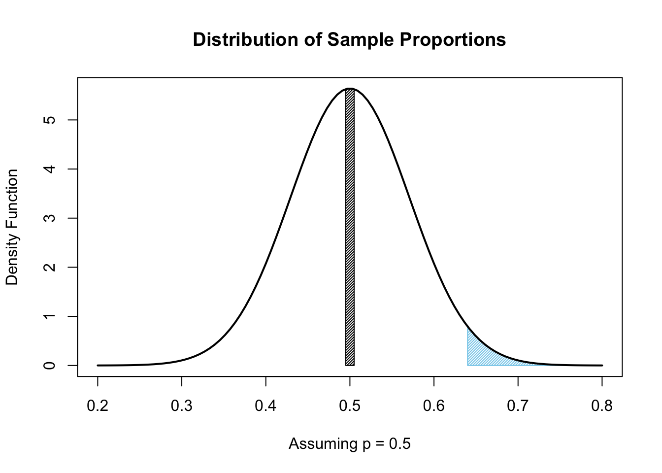
Figure 9.7: One-Tailed Plot

The black vertical bar is a graphical reminder of what we expect $\hat{p}$ to be, because $\mu_{\hat{p}} = p = 0.5$ by assumption. The area bounded by the entire curve is 1, just like any other Density Function, and the area of the blue shaded region represents the probability that a random sample would give $\hat{p} \geq 0.64$.

Another way of stating this is that if we assume that $p = 0.5$, then only 2.4% of random samples would give a $\hat{p}$ at least as extreme as the sample (evidence) we have. To return to our courtroom analogy, this would be equivalent to saying that the evidence presented against a defendant would also point towards approximately 2.4% of all people. That is, 1 in about every 40 people would appear just as guilty as the accused. Is this sufficient evidence to reject our assumption of innocence and find the defendant not guilty? We will return to this in a moment when we discuss what threshold we should use when doing this sort of analysis.

Above, we only considered samples with a $z$-statistic more than 1.979899. What if we also considered samples which were as equally extreme, but have $\hat{p}<0.5$. That is, we consider samples whose $z$-statistics are such that

\[ z < -1.979899 \;\; \text{ or } \;\; z > 1.979899\]

We can find the probability of a random sample having such a $z$-statistic with qnorm once again.

pnorm( q = -1.979899, lower.tail = TRUE ) + pnorm( q = 1.979899, lower.tail = FALSE )

## [1] 0.04771488

That is, we expect about 4.8% of samples to have a $\hat{p}$ that is extreme as the one we observed in either direction from $p = 0.5$. We can once again visualize this with a graph.

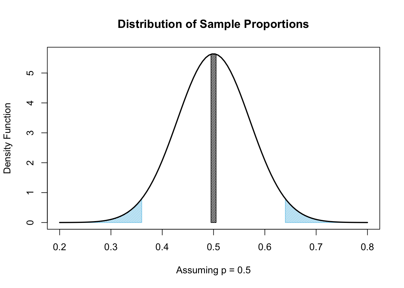
Figure 9.8: Two-Tailed Plot

Here the blue area is approximately 0.048 and this graph gives a nice visual argument that our new probability is exactly twice that of our previous one.

We can verify this fact with the reminder that the standard Normal distribution has a symmetric density function about $z = 0$ so that for a positive value of $z_0$ we get that $P( X > z_0) = P( X < -z_0)$.

It is clear that we have two different percentages which are supposed to be our evidence against $H_0: p = 0.5$. We could try to prove that $p > 0.5$ or simply try to prove that $p \neq 0.5$ based on our evidence of $\hat{p}_0 = 0.64$. In the first case where we only considered samples as extreme and on the same side of $p$, we set the alternative hypothesis, denoted $H_a$, to be $p > 0.5$. Thus, we have the following two hypotheses in this case.

\[\begin{align*} H_0 &: p = 0.5\\ H_a &: p > 0.5 \end{align*}\]

In this scenario our graph had only a single blue tail and we call this a One-Tailed Hypothesis Test. The strength of the evidence of our estimate is what we call the $p$-value.

Remark. The following definition is an interpretation of the “informal” definition of a $p$-value as given by the American Statistical Association¹⁰². Unfortunately, a rigorous definition is not easily given, nor is its interpretation fully agreed upon.

Definition 9.10 A $p$-value is the probability, under the assumptions of a hypothesis test, that a statistic from a random sample (from the same distribution as the observed sample) would be equal to or more extreme than the observed value of the statistic.

In our case, we get that $p\text{-value} \approx 0.024$. That is, there is approximately a 2.4% chance that a random sample of 50 coin flips will result in a sample with $\hat{p} \geq \frac{32}{50}$.

Definition 9.11 The hypotheses for a One-Tailed Hypothesis Test of a population proportion will always be one of the forms below where $p_0$ is simply a placeholder for the assumed value of the population proportion.

\[\begin{align*} H_0 &: p = p_0\\ H_a &: p > p_0 \end{align*}\]

\[\begin{align*} H_0 &: p = p_0\\ H_a &: p < p_0 \end{align*}\]

It is important to not confuse the different uses of $p$ here. We have a population proportion which we denoted $p$ and now a measure of how strong evidence based on a sample which we call the $p$-value. We also use $P$ for probability calculations, $\hat{p}$ for a sample proportion, and even $\hat{p}_0$ for an observed sample proportion. Due to the plethora of “p”s, we will always write out $p$-value to avoid confusion as much as possible.

Remark. Some sources will write $H_0$ as $p \leq p_0$ when the alternative is $p > p_0$ and similarly write $H_0: p \geq p_0$ when $H_a: p < p_0$. This is simply a choice, but the version used here makes it clear what value should be used within any calculations.

Loosely, we can take the $p$-value to represent how much you can still believe the assumption made in $H_0$ after examining the evidence against it. If we absolutely believe in the statement(s) made in $H_0$ prior to running the test, then we can view $p$-value as how much belief we still have in after examining the evidence provided by our sample. We will soon discuss how little belief is acceptable before we are forced to reject $H_o$. However, it is important to also remember that this is just a loose way to make sense of it and that the technical meaning is given in Definition 9.10.

If we look at the second version of the analysis where our graph had two tails, it makes sense that here we are giving evidence for $p \neq 0.5$ (as compared to the more strict $p>0.5$ we used before). In this case, we have the following set of hypotheses.

\[\begin{align*} H_0 &: p = 0.5\\ H_a &: p \neq 0.5 \end{align*}\] We call this a Two-Tailed Hypothesis Test. In this case, we get that $p\text{-value} \approx 0.048$.

Definition 9.12 The hypotheses for a Two-Tailed Hypothesis Test of a population proportion will always be of the form below where $p_0$ is simply a placeholder for the assumed value of the population proportion.

\[\begin{align*} H_0 &: p = p_0\\ H_a &: p \neq p_0 \end{align*}\]

Remark. If all other factors are kept the same, the $p$-value for a two-tailed hypothesis test will always be twice that of the the $p$-value for a one-tailed test. In practice, nearly all hypothesis tests done are two-tailed as doing a one-tailed hypothesis test can be viewed as a very simple example of what is called $p$-hacking or Data Dredging because it will always result in a lower $p$-value.¹⁰³

Most¹⁰⁴ hypothesis tests we will look at in Statypus will be of the following form:

\[\begin{array}{c|c} H_0 : \text{True Parameter} = \text{Assumed Paramter} &\text{Assumed Situation}\\ H_a : \text{True Parameter} \; \Box \;\text{Assumed Paramter} &\text{Claim Being Tested} \end{array}\]

where $\Box \in \left\{<, >,\neq \right\}$ and is chosen so that \[\text{Sample Statistic} \; \Box \; \text{Assumed Paramter}\] is true.

We assume the information in $H_0$ but are attempting to prove the claim made by $H_a$.

If our $p$-value is low enough (based on the level of significance which we will introduce in Section 9.3.5 ) we can then abandon the assumption and can say that we have “proven”¹⁰⁵ the claim.

9.3.3 The Code for Hypothesis Tests

The following code will run a hypothesis test based on the user entered values.

x =                #Number of "Good" cases
n =                #Sample Size
p0 =               #Value of p in null hypothesis
Tails =            #The number of tails: Either 1 or 2
#Below here is stock code and should not be changed
pHat0 <- x / n     #Sample proportion
SD <- sqrt( p0 * ( 1 - p0 ) / n )
zStat <- ( pHat0 - p0 ) / SD
pValue <- Tails*pnorm( q = - abs( zStat ) )   
pValue

Example 9.17 We can use the “Unfair Coin” from Example 9.15 to see how this code template works.

x = 32            #Number of "Good" cases
n = 50            #Sample Size
p0 = 0.5          #Value of p in null hypothesis
Tails = 1         #The number of tails: Either 1 or 2
#Below here is stock code and should not be changed
pHat0 <- x / n    #Sample proportion
SD <- sqrt( p0 * ( 1 - p0 ) / n )
zStat <- ( pHat0 - p0 ) / SD
pValue <- Tails*pnorm( q = - abs( zStat ) )   
pValue

## [1] 0.02385744

We now know how to interpret this value. We know that only 2.4% of samples of 50 flips of a fair coin would produce a sample proportion that is as high or higher than our observed value, $\hat{p}_0 = \frac{32}{50}$. Whether or not this $p$-value is low enough (i.e. sufficient evidence) will be determined on where we set our threshold. We will get to that shortly.

We will do this now with the second version of our analysis of the coin where we had $H_a: p \neq 0.5$. The only change we make here is we change the value of Tails to be 2.

x = 32            #Number of "Good" cases
n = 50            #Sample Size
p0 = 0.5          #Value of p in null hypothesis
Tails = 2         #The number of tails: Either 1 or 2
#Below here is stock code and should not be changed
pHat0 <- x / n    #Sample proportion
SD <- sqrt( p0 * ( 1 - p0 ) / n )
zStat <- ( pHat0 - p0 ) / SD
pValue <- Tails*pnorm( q = - abs( zStat ) )   
pValue

## [1] 0.04771488

This says that a fair coin would produce a sample proportion that is more extreme in either direction (i.e. favoring heads or tails) approximately 4.8% of the time. Again, we will leave the decision of how to finally interpret this value until we have set a threshold.

9.3.4 The Boy Who Cried Wolf

The Boy Who Cried Wolf¹⁰⁶ is one of Aesop’s Fables and a classic allegory read to many children.¹⁰⁷ The fable is based on a young shepherd boy guarding a village’s sheep on a hill. It was the boy’s job to inform the village people if a wolf were to appear so that the villagers could fended off the wolf and protect the sheep. The villagers lived their lives under the assumption that there were no wolves on the hill unless the shepherd boy alerted them to the danger. However, the boy becomes bored (and possibly lonely) and he cries “Wolf! Wolf!” to illicit a response from the village. The villagers came rushing only to find that the boy was laughing at how he had fooled them. After fooling the townspeople with another fake cry of “Wolf! Wolf!”, the villagers become upset with the boy and returned to the village no longer trusting the boy. Later, when a wolf did appear, the boy again tried to call for the villagers and the villagers simply ignored his cry and did not come to his aid assuming the boy was once again telling a lie. The wolf scattered the sheep and one version of the fable ends with the moral of “Liars are not believed even when they speak the truth.”

Now, it is good to question why this classic fable is being recounted here. However, it is a great way of keeping the two different errors that can result from a hypothesis test straight.

We can view the villagers as running a hypothesis test where they live under the assumption that there are no wolves, $H_0$, while they also listen for evidence from the boy that there are wolves, $H_a$. That is, we can view anytime that the boy cries wolf as a hypothesis test with the following hypotheses.

\[\begin{align*} H_0 &: \text{Wolves} = 0\\ H_a &: \text{Wolves} > 0 \end{align*}\]

Now, for this or any hypothesis test, there are two different errors we could make. As our two outcomes of a hypothesis test is to reject $H_0$ (thought of as a Guilty sentence) or fail to reject $H_0$ (thought of as a Not Guilty sentence).

Definition 9.13 If we reject $H_0$ when it was valid, this is known as a Type I Error. This is analogous to a court wrongfully convicting an innocent man.

If we fail to reject $H_0$ when it is invalid, this is known as a Type II Error. This is analogous to letting a guilty person go free.

This setup of the types of error do show a bit of a conundrum. If we try to minimize the probability of convicting an innocent person, then we automatically increase the probability of letting a guilty person go free. In the next section, we will talk about the probability of making a Type I Error.

In the context of the shepherd boy, a Type I Error would be equivalent to the townspeople finding the boy’s cry sufficient evidence to abandon $H_0 : \text{Wolves} = 0$ and conclude $H_a : \text{Wolves} > 0$ when, in fact, there are no wolves. This is precisely the villagers make repeated times early in the fable.

A Type II Error would occur when the villagers heard the boy crying wolf and neglected to believe his cries and thus did not abandon their assumption of $H_0 : \text{Wolves} = 0$ when there indeed was a wolf threatening the sheep.

The first type of error that the villagers make in The Boy Who Cried Wolf is a Type I Error and the second type of error they make is a Type II Error.

9.3.5 Using an Alpha Value

We have still not yet decided at what point a $p$-value becomes so low that we will conclude that the evidence is sufficient to abandon our assumption made in $H_0$. It seems clear that we need a threshold, $\alpha$, called the level of significance or significance level, that when $p\text{-value}< \alpha$ that we conclude that we have sufficient evidence to reject $H_0$.

A very common standard is to set $\alpha = 0.05$. By choosing this, what we have done is to set the probability of making a Type I error to be 5%.

Definition 9.14 The chosen value of $\alpha$ is the probability of making a Type I error when conducting a hypothesis test and is called the Level of Significance.

Remark. There is a bit of push back against such a rigid choice of $\alpha = 0.05$ and many introductory textbooks do also consider options such as $\alpha = 0.01$. However, setting any fixed value of $\alpha$ can be seen as narrow minded.¹⁰⁸

The American Statistical Association made this statement in an article.

Scientific conclusions and business or policy decisions should not be based only on whether a p-value passes a specific threshold. Practices that reduce data analysis or scientific inference to mechanical “bright-line” rules (such as “$p$ < 0.05”) for justifying scientific claims or conclusions can lead to erroneous beliefs and poor decision making. A conclusion does not immediately become “true” on one side of the divide and “false” on the other. Researchers should bring many contextual factors into play to derive scientific inferences, including the design of a study, the quality of the measurements, the external evidence for the phenomenon under study, and the validity of assumptions that underlie the data analysis. Pragmatic considerations often require binary, “yes-no” decisions, but this does not mean that $p$-values alone can ensure that a decision is correct or incorrect. The widespread use of “statistical significance” (generally interpreted as “$p \leq 0.05$”) as a license for making a claim of a scientific finding (or implied truth) leads to considerable distortion of the scientific process.

Definition 9.15 An observed sample is said to be statistically significant at the level of significance if its $p$-value in a hypothesis test is no more than $\alpha$. If $p$-value>$\alpha$, we say that the sample is not statistically significant at the level of significance.

Now that we have all of our terminology, formulas, and code setup, we can explicitly define what the conclusions of a hypothesis test are.

Definition 9.16 When an observed sample is statistically significant for a particular $\alpha$, then we have found Sufficient Evidence to reject the assumption in the null hypothesis and can accept the claim being made in the alternative hypothesis (at that level of significance).

When an observed sample is not statistically significant, than we have found Insufficient Evidence to reject the assumption in the null hypothesis and cannot accept the claim being made in the alternative hypothesis (at that level of significance). In this case, the hypothesis test has NOT proven $H_0$ and we simply have failed to reject it.

Remember, you cannot prove something that was assumed!

The following exploration gives a visual way of interpreting a hypothesis test. If we imagine our belief in $H_0$ to be the length of the spring, then due to our assumption, it begins with a length of 1 as shown. If the evidence can supply sufficient evidence, it will compress the spring so that its entire lenght lies within the purple region. If the top of the spring (visualized by the green bar) remains in the blue region, however, then the evidence is not sufficient and we can not reject the null hypothesis.

You can adjust the $\alpha$ value by using the orange dot on the left side of the box and then drag the slider below the box to set the $p$-value to what was found.

If the green bar is in the blue region, we have insufficient evidence and cannot reject our assumption made in $H_0$.
If the green bar is in the purple region, we have sufficient evidence to reject $H_0$ and can claim to have proven $H_a$ at the $\alpha$ level of significance.

A quick example (with the calculations omitted) of why a static value of $\alpha = 0.05$ can be viewed as silly is as follows.

Example 9.18 If we have a sample where 321 out of 500 respondents are female, we get $\hat{p}_0 = 0.642$. If we were to test the hypothesis of $p \neq 0.6$, then we get a $p$-value of 0.05523 which is larger than $\alpha = 0.05$ so we would be unable to abandon our assumption that $p = 0.6$.

However, if even a single other person in the sample were to be female, we would now have $x = 322$ and we get $p\text{-value} \approx 0.04461 < \alpha = 0.05$ and we would be justified to conclude that we have sufficient evidence at the $\alpha = 0.05$ level of significance to reject $H_0: p = 0.6$ and conclude that $p \neq 0.6$.

This example is important to illustrate that a study should definitely give their $p$-value instead of just stating how it compares to $\alpha$. Our sample with 321 females was insufficient proof of $p \neq 0.6$, but it was very close to being sufficient. Meanwhile, a sample with 322 females out of 500 was sufficient evidence to conclude $p \neq 0.6$.

There is no consensus on the best way to handle this in general and in this book we may simply consider a generic value of $\alpha$ and set an actual value when an example requires an explicit answer.

9.3.6 Applications of Hypothesis Test for Population Proportion

Example 9.19 (The Unfair Coin Returns) We return, once again, to the scenario of the Unfair Coin introduced in Example 9.15. If we were to set $\alpha = 0.05$ as our level of significance, then in Example 9.17 we found sufficient evidence to abandon our assumption that $p =0.5$ (i.e. that the coin is fair) and conclude that either $p \neq 0.5$ ($p\text{-value} \approx 0.024$) or more strongly that $p > 0.5$ ($p\text{-value} \approx 0.048$). That is, a sample of 32 heads out of 50 flips of a coin gives sufficient evidence at the $\alpha = 0.05$ level of significance to reject the assumption of $H_0$, $p=0.5$, and we are justified in believing the claim of the alternative hypothesis that states $p>0.5$ (or simply $p\neq 0.5$).

Example 9.20 (The Reckoning of Melody) Earlier, we saw that Melody had a success rate of $\frac{13}{40} = 0.325$ for putting her shoes on the correct feet. We want to finally decide how the evidence we gathered earlier in the form of a confidence interval can be regarded as “proof” that Melody’s actual “population” proportion was not 0.5.

We can choose to try and prove that she is simply not an ape, $H_a: p \neq 0.5$, or if she is in fact performing worse than a blind ape in a dark room, $H_a: p < 0.5$. We begin with the one-tailed test below.

x = 13            #Number of "Good" cases
n = 40            #Sample Size
p0 = 0.5          #Value of p in null hypothesis
Tails = 1         #The number of tails: Either 1 or 2
#Below here is stock code and should not be changed
pHat0 <- x / n    #Sample proportion
SD <- sqrt( p0 * ( 1 - p0 ) / n )
zStat <- ( pHat0 - p0 ) / SD
pValue <- Tails*pnorm( q = - abs( zStat ) )   
pValue

## [1] 0.01342835

So, for our one-tailed test, we get a $p$-value of approximately 1.3%. This does pass the criteria that $p\text{-value}<\alpha = 0.05$, but are we ready to abandon our assumption that she was at least as capable as a BADR and conclude we have proven that she performs worse? To give her the best chance at being acquitted, we can also perform the two-tailed test below.

x = 13            #Number of "Good" cases
n = 40            #Sample Size
p0 = 0.5          #Value of p in null hypothesis
Tails = 2         #The number of tails: Either 1 or 2
#Below here is stock code and should not be changed
pHat0 <- x / n    #Sample proportion
SD <- sqrt( p0 * ( 1 - p0 ) / n )
zStat <- ( pHat0 - p0 ) / SD
pValue <- Tails*pnorm( q = - abs( zStat ) )   
pValue

## [1] 0.0268567

For our two-tailed test, we get a $p$-value of approximately 2.6%. Sadly, this means that even the most favorable test, we get that we should only expect a sample as extreme as Melody’s one out of roughly every 40 times.

If we choose that $\alpha = 0.05$, then sadly, we must reject our null hypothesis in both versions of our hypothesis test and would claim we had sufficient evidence to conclude that $p \neq 0.5$ or moreover that $p < 0.5$.

However, if we choose that $\alpha = 0.01$, then in either hypothesis test, we have insufficient evidence to abandon our assumption and would be unable to justify the claims made in $H_a$. This mirrors the results we had for the confidence intervals where a 95% Confidence Interval did not contain 0.5, but a 99% Confidence Interval did.

At this point, we are best to simply state our $p$-value of either approximately 1.3% or 2.6% and let the reader make their own decision about what to conclude about the hypotheses. However, regardless of what statistical result you choose to make, the author implores you to reserve judgement on Melody as a little girl until having read Section 9.4.

Remark. The above example is crucial to understand. It shows that the conclusion of a hypothesis test depends not only on the hypotheses and observed sample, but also the choice of $\alpha$. The hypothesis tests about Melody’s shoes showed that we had sufficient evidence to abandon $H_0$ when $\alpha = 0.05$ but insufficient evidence when $\alpha = 0.01$.

Example 9.21 (b vs g Revisited) Earlier we were investigating the proportion of US babies that are born female. We saw the number of boys born in the US in 2000 was 2,076,969 and the number of girls born was 1,981,845. If we move to test whether the underlying population proportion, $p$, was actually less than 0.5 based on this evidence, we can run the following hypothesis test.

\[\begin{align*} H_0 &: p = 0.5\\ H_a &: p < 0.5 \end{align*}\]

We can do this with the following code.

b = 2076969
g = 1981845
x = g             #Number of "Good" cases
n = b+g           #Sample Size
p0 = 0.5          #Value of p in null hypothesis
Tails = 1         #The number of tails: Either 1 or 2
#Below here is stock code and should not be changed
pHat0 <- x / n    #Sample proportion
SD <- sqrt( p0 * ( 1 - p0 ) / n )
zStat <- ( pHat0 - p0 ) / SD
pValue <- Tails*pnorm( q = - abs( zStat ) )   
pValue

## [1] 0

This gives a $p$-value that is so small that it is smaller than the smallest positive number that R can work with. This number¹⁰⁹ is exceptionally low and far below any $\alpha$ value we will ever look at.

That is, we have sufficient evidence that the proportion of US baby girls is less than 0.5.

A natural question is then, what is the proportion of girls born in the US? Our 2000 sample would lead us to believe that there are approximately 1.05 non females born for every 10 girls. That is, we would expect 20 out of every 41 babies to be born a female. We can test if we have sufficient evidence to even abandon this value of $p$ by making only slight modifications to the code above.

b = 2076969
g = 1981845
x = g             #Number of "Good" cases
n = b+g           #Sample Size
p0 = 20/41        #Value of p in null hypothesis
Tails = 2         #The number of tails: Either 1 or 2
#Below here is stock code and should not be changed
pHat0 <- x / n    #Sample proportion
SD <- sqrt( p0 * ( 1 - p0 ) / n )
zStat <- ( pHat0 - p0 ) / SD
pValue <- Tails*pnorm( q = - abs( zStat ) )   
pValue

## [1] 0.05457713

This shows that our sample gave sufficient evidence to confidently concluded that $p < 0.5$, but it fails to give sufficient evidence to the the fact that $p \neq \frac{20}{41}$. In fact, this ratio (usually reported as the number of boys for every thousand girls) is well studied and can take on different values in different countries.¹¹⁰

9.4 Part 4: The Redemption of Melody

Figure 9.9: Our Favorite Little Blondie

Up until now, it may have seemed like we have been unfairly harsh to the little blonde girl, Melody. However, there is a nice conclusion to this story. It is important to recall we are discussing a very intelligent and head strong little girl. Melody was fiercely independent with some things and her shoes were certainly one of them. She would grab her shoes and run off to a corner and not return until her shoes were on her feet.

Melody was definitely trying her best to get her shoes on the correct feet, but something was definitely encumbering those attempts. What was going on?

We have to try to think like a little girl to fully understand what was going on. If you have a shoe somewhere nearby grab it, just one will do.

Seriously, grab a shoe.

Look at the shoe from its top side. As adults, we are quite adept at looking at a shoe like this and easily realizing which foot it should go on. However, turn the shoe over and you will see that the curvature of it is far more apparent from the bottom. As a young person learning how to tell the shoes apart, it makes a lot of sense to look at the bottom and try to decide which foot that shoe should go on.

If you are holding a left shoe and turn it over to look at the bottom of the shoe, what do you see? Moreover, if you tried to match this shoe to one of your feet, which foot would it match?

If you try this, it should become clear that as we look at the bottom of a left shoe that the sole of the shoe would align with the curvature of our right foot!

Melody was turning her shoes over and matching them to her feet!

While this may seem like an obviously flawed strategy to an adult, given enough compassion, it is fair to say that for a young learner, this strategy is well thought out and far more rational than blind apes guessing in dark rooms. Unfortunately, our feet, and thus our shoes are chiral objects.¹¹¹ The chirality of our feet, shoes, hands, arms, and legs is a logical inconvenience that as adults we have typically overcome. However, this little girl was literally learning the concept of chirality with her trial and error, and if you ask Melody the question “How do we learn?”, she will undoubtedly say “By making mistakes.”

It only took one very brief conversation with Melody to finally demystify the difficulty she was having. She quickly grasped the concept and was so excited to demonstrate that she now understood it!

As learners, it is so important to realize that even repeated mistakes can often be the path to a true and deep understanding of a concept.

9.5 Part 5: `binom.test`

We have learned to leverage the power of the R software to reduce the burden of tedious calculations. Modern statistics, data science, and analytics involves the mindset of being aware and conscious of what the machine is doing, but leveraging the computation power we now have to be able to analyze massive data sets. With this view, it may seem odd that we had to basically conduct the analysis “by hand” for all of the stuff in this chapter. It seems there should be an easier way to handle confidence intervals and hypothesis tests for a population proportion.

This is indeed the case. We can use the function, binom.test(), to do all of the above calculations. In fact, binom.test makes exact binomial calculations without the need to invoke the Central Limit Theorem, which we used at the beginning of this chapter. While the results will not match our previous efforts perfectly, they will be very close and, in fact, better.

Remark.

If the choice of methods (by hand versus binom.test) were to affect the results of a hypothesis test for some significance level, it would be appropriate to explicitly mention the technique(s) being used and be skeptical to express the result as being conclusive.
The lack of consistent results among different methods dovetails in precisely with our conversation about the awkwardness of setting a strict arbitrary threshold of $\alpha$.
It is worthy to mention that the output from binom.test will likely not match solutions shown in other introductory statistics books or homework systems.

9.5.1 Code for `binom.test`

The syntax of binom.test() is

binom.test( x, n, p, alternative, conf.level )     
#This code will not run unless the necessary values are inputted.

where the parameters are:

x: Count of successes.
n: Number of trials.
p: The assumed value of the population proportion in the hypothesis test you are running. By default, p = 0.5. Not needed for confidence intervals.
alternative: The symbol in the alternative hypothesis in a hypothesis test. Must be one of "two.sided", "less", and "greater". DO NOT USE for confidence intervals.
conf.level: The confidence level for the desired confidence interval. Not needed for hypothesis test.

Note: alternative is set to "two.sided" by default if you do not enter this parameter.

Example 9.22 (The Unfair Coin Revisited Again) We now revisit the “Unfair Coin,” first discussed in Example 9.15 and last seen in Example 9.19, using binom.test. Using the syntax above, we get the following output from binom.test for a 95% confidence interval.

binom.test( x = 32, n = 50, conf.level = 0.95 )

## 
##  Exact binomial test
## 
## data:  32 and 50
## number of successes = 32, number of trials = 50, p-value = 0.06491
## alternative hypothesis: true probability of success is not equal to 0.5
## 95 percent confidence interval:
##  0.4919314 0.7708429
## sample estimates:
## probability of success 
##                   0.64

We compare this to the manual versions using the code chunks we developed earlier.

#Confidence Interval Code
x = 32              #Number of "Good" cases
n = 50              #Sample Size
C.Level = 0.95      #Confidence Level
#Only change values above this line
pHat0 <- x / n      #Sample proportion
SE <- sqrt( pHat0 * (1 - pHat0) / n )
zStar <- qnorm( 1 - (1 - C.Level) / 2 )
MOE <- zStar * SE
CIL <- pHat0 - MOE  #Confidence Interval Lower Bound
CIU <- pHat0 + MOE  #Confidence Interval Upper Bound
c( CIL, CIU )       #Confidence Interval

## [1] 0.5069532 0.7730468

While our manual technique yielded a 95% Confidence Interval of roughly $( 0.507, 0.773)$, we see that binom.test gives an interval of $( 0.492, 0.771 )$. With binom.test we cannot say that we are 95% confident that $p>0.5$!

The manual technique gives a margin of error of approximately 0.133 while binom.test gives a margin of error of roughly 0.139. The higher powered binom.test is not forced to be centered on the value of $\hat{p}_0$ being that it uses discrete (based on the size of $n$) techniques, but it does offer a larger margin of error compared to the manual techniques for the same confidence.

Remark. The function binom.test finds confidence intervals that have confidence at least the level the user specifies and often surpasses it.¹¹²

We can pivot and conduct the one-tailed hypothesis test run in Example 9.19, but now with binom.test.

binom.test( x = 32, n = 50, p = 0.5, alternative = "greater")

## 
##  Exact binomial test
## 
## data:  32 and 50
## number of successes = 32, number of trials = 50, p-value = 0.03245
## alternative hypothesis: true probability of success is greater than 0.5
## 95 percent confidence interval:
##  0.5142308 1.0000000
## sample estimates:
## probability of success 
##                   0.64

To understand any changes, we remind the reader of our results from before.

x = 32            #Number of "Good" cases
n = 50            #Sample Size
p0 = 0.5          #Value of p in null hypothesis
Tails = 1         #The number of tails: Either 1 or 2
#Below here is stock code and should not be changed
pHat0 <- x / n    #Sample proportion
SD <- sqrt( p0 * ( 1 - p0 ) / n )
zStat <- ( pHat0 - p0 ) / SD
pValue <- Tails*pnorm( q = - abs( zStat ) )   
pValue

## [1] 0.02385744

Manual techniques give a $p$-value of $0.024$ (as we saw before), but binom.test gives a $p$-value of $0.032$. This shows that using the manual techniques of using the Central Limit Theorem gives a $p$-value lower than is absolutely necessary.

We can finally compare the manual two-tailed analysis to the result from binom.test.

x = 32            #Number of "Good" cases
n = 50            #Sample Size
p0 = 0.5          #Value of p in null hypothesis
Tails = 2         #The number of tails: Either 1 or 2
#Below here is stock code and should not be changed
pHat0 <- x / n    #Sample proportion
SD <- sqrt( p0 * ( 1 - p0 ) / n )
zStat <- ( pHat0 - p0 ) / SD
pValue <- Tails*pnorm( q = - abs( zStat ) )   
pValue

## [1] 0.04771488

binom.test( x = 32, n = 50, p = 0.5, alternative = "two.sided" )

## 
##  Exact binomial test
## 
## data:  32 and 50
## number of successes = 32, number of trials = 50, p-value = 0.06491
## alternative hypothesis: true probability of success is not equal to 0.5
## 95 percent confidence interval:
##  0.4919314 0.7708429
## sample estimates:
## probability of success 
##                   0.64

This shows that at the $\alpha = 0.05$ level of significance the manual techniques would have concluded that 32 heads out of 50 flips was sufficient evidence to abandon the assumption that $p=0.5$ and conclude that $p \neq 0.$. However, binom.test shows that 32 heads out of 50 flips is NOT sufficient evidence to reject $H_0: p=0.5$!

The exact calculations of binom.test for both confidence intervals and hypothesis tests should be considered superior to that of the manual techniques. However, as we have just seen, making this switch to using the Exact Binomial Test may cause a result that was statistically significant to not be statistically significant anymore.

9.5.2 Applications with `binom.test`

Example 9.23 (Confidence Intervals for b vs.g) We can redo the calculations made in Examples 9.13 and 9.21 using binom.test. We begin by looking at confidence intervals with the different confidence intervals we used in Example 9.13. Note that conf.level changes each time.

b = 2076969
g = 1981845
binom.test( x = g, n = b + g, conf.level = 0.9)

## 
##  Exact binomial test
## 
## data:  g and b + g
## number of successes = 1981845, number of trials = 4058814, p-value < 2.2e-16
## alternative hypothesis: true probability of success is not equal to 0.5
## 90 percent confidence interval:
##  0.4878736 0.4886900
## sample estimates:
## probability of success 
##              0.4882818

binom.test( x = g, n = b + g, conf.level = 0.95)

## 
##  Exact binomial test
## 
## data:  g and b + g
## number of successes = 1981845, number of trials = 4058814, p-value < 2.2e-16
## alternative hypothesis: true probability of success is not equal to 0.5
## 95 percent confidence interval:
##  0.4877954 0.4887682
## sample estimates:
## probability of success 
##              0.4882818

binom.test( x = g, n = b + g, conf.level = 0.999)

## 
##  Exact binomial test
## 
## data:  g and b + g
## number of successes = 1981845, number of trials = 4058814, p-value < 2.2e-16
## alternative hypothesis: true probability of success is not equal to 0.5
## 99.9 percent confidence interval:
##  0.4874653 0.4890984
## sample estimates:
## probability of success 
##              0.4882818

These values match nearly precisely with the manual calculations we made earlier.

We can also use binom.test to complete the hypothesis test for $P(g)$ with $p_0 = 0.5$ that we ran in Example 9.21.

binom.test( x = g, n = b + g, p = 0.5 )

## 
##  Exact binomial test
## 
## data:  g and b + g
## number of successes = 1981845, number of trials = 4058814, p-value < 2.2e-16
## alternative hypothesis: true probability of success is not equal to 0.5
## 95 percent confidence interval:
##  0.4877954 0.4887682
## sample estimates:
## probability of success 
##              0.4882818

Like before, we get a $p$-value that is essentially zero and thus we have sufficient evidence at any reasonable level of significance to conclude that the true proportion of girls is not 0.5.

We can also use binom.test to run the hypothesis test for $P(g)$ with $p_0 = \frac{20}{41}$.

binom.test( x = g, n = b + g, p = 20/41 )

## 
##  Exact binomial test
## 
## data:  g and b + g
## number of successes = 1981845, number of trials = 4058814, p-value = 0.05461
## alternative hypothesis: true probability of success is not equal to 0.4878049
## 95 percent confidence interval:
##  0.4877954 0.4887682
## sample estimates:
## probability of success 
##              0.4882818

This gives a $p$-value that is just slightly higher than our manual calculations gave in Example 9.21. Regardless, at the $\alpha = 0.05$ level of significance (or any stricter level), we have insufficient evidence to abandon the assumption that $p = \frac{20}{41}$.

Example 9.24 (The Return of The Melody) We can also reevaluate Melody’s situation using binom.test. We first give the code for the confidence interval.

binom.test( x = 13, n = 40, conf.level = 0.95 )

## 
##  Exact binomial test
## 
## data:  13 and 40
## number of successes = 13, number of trials = 40, p-value = 0.03848
## alternative hypothesis: true probability of success is not equal to 0.5
## 95 percent confidence interval:
##  0.1857290 0.4912949
## sample estimates:
## probability of success 
##                  0.325

This gives a confidence interval of $(0.1857290 0.4912949)$ which is slightly wider than the interval we found in Example 9.14,$(0.1798518, 0.4701482)$. Recall that that binom.test actually finds intervals that have a confidence level that is often higher than we explicitly ask of it.

We now give the code for the hypothesis test where the alternative hypothesis is given by $H_a: p < 0.5$.

binom.test( x = 13, n = 40, p = 0.5, alternative = "less" )

## 
##  Exact binomial test
## 
## data:  13 and 40
## number of successes = 13, number of trials = 40, p-value = 0.01924
## alternative hypothesis: true probability of success is less than 0.5
## 95 percent confidence interval:
##  0.0000000 0.4662951
## sample estimates:
## probability of success 
##                  0.325

This gives a $p$-value of 0.01924 which is significantly closer to the proportion of blind apes that succeeded no more often than Melody did, 0.1930, in our simulation of one million blind apes in Section 8.4 than the value we found earlier, which was 0.01343. That value (0.01343) matches with the value we found for $P( \hat{p} \leq 0.325 )$ earlier.

9.5.3 Conditions for Inference on a Population Proportion

THIS SECTION HAS YET TO BE WRITTEN

Theorem 9.7 The sample was gathered with care given to minimize all possible bias and to ensure the sample is as representative of the population as is possible.

9.6 Part 6: Inference of Multiple Population Proportions

As we mentioned in Chapter 5, it is often helpful to look at the relationship between two populations and not just the individual populations in isolation. In this section, we want to investigate population proportions coming from (at least)¹¹³ two different populations, $p_1$ and $p_2$. To investigate these two parameters, we need to start by collecting two samples and obtaining two statistics, sample proportions in this case. For us this means we need values of the form

\[\hat{p}_k = \frac{x_k}{n_k} \;\text{ for } k = 1,2.\] As we have seen, what we now have statistics that are point estimates of parameters. That is,for $k = 1,2$, we have

\[\begin{align*} \text{Statistic} &\approx \text{Parameter}\\ \hat{p}_k &\approx p_k. \end{align*}\]

We know that the each distribution of the values of $\hat{p}_k$ follows

\[\text{Norm}\left(\mu_{\hat{p}_k} , \sigma_{\hat{p}_k} \right),\]

where

\[\begin{align*} \mu_{\hat{p}_k} &= p_k \text{ and }\\ \sigma_{\hat{p}_k} &= \sqrt{ \frac{ p_k(1-p_k)}{n_k}}, \end{align*}\]

but we don’t know what the distribution of values of form \[\hat{p}_1 - \hat{p}_2\] would follow. This is given in the following theorem.

Theorem 9.8 If we have two independent samples drawn from distributions that each satisfy the conditions of Theorem 8.2, then the distribution of values of $\hat{p}_1 - \hat{p}_2$ follows a roughly Normal distribution with the following parameters.

\[\begin{align*} \mu_{\hat{p}_1 - \hat{p}_2} &= p_1 - p_2\\ \sigma_{\hat{p}_1 - \hat{p}_2} &= \sqrt{ \sigma_{\hat{p}_1}^2 + \sigma_{\hat{p}_2}^2 } \end{align*}\]

Remark. We will not get too formal about the definition about independent here, but the essence is that the selection of one sample should not have any impact on the selection of the other.

From this we could obtain a $z$-statistic to conduct a hypothesis test of form

\[\begin{align*} H_0 &: p_1 - p_2 = p_0\\ H_a &: p_1 - p_2 \;\Box\; p_0 \end{align*}\]

via the formula below \[z = \frac{ \left(\hat{p}_1 - \hat{p}_2\right) - \mu_{\hat{p}_1 - \hat{p}_2}}{ \sigma_{\hat{p}_1 - \hat{p}_2}}\] where $p_0$ is some unknown difference in the population proportions and $\Box$ is one of the symbols $<$, $>$, or $\neq$.

If we wish to obtain a confidence interval, we could approximate the standard deviation with a standard error, $\text{SE}$, which is given below and compute a Margin Of Error by also using a $z^*$ value.

\[\sigma_{\hat{p}_1 - \hat{p}_2} \approx \text{SE} = \sqrt{ \frac{ \hat{p}_1(1-\hat{p}_1)}{n_1} + \frac{ \hat{p}_2(1-\hat{p}_2)}{n_2}}\]

9.6.1 `prop.test`

This is typically where we would setup a Code Template that would run the above calculations for either a hypothesis test or confidence interval. However, in this instance, we will simply comment that this method is definitely possible, but one that we will not use here on Statypus. We saw the power of binom.test in Section 9.5 and how it was able to handle all problems for one sample population proportion inference and even offer us stronger results by applying stronger methods.

It would be amazing if binom.test could simply be used here to provide information when we are dealing with two sample proportions, but sadly it cannot. However, there is another base R function that fits the bill perfectly, prop.test().

The syntax of prop.test() is

prop.test( x, n, p, alternative, conf.level, correct )     
#This code will not run unless the necessary values are inputted.

where the parameters are:

x: A vector of counts of successes.
n: A vector of number of trials.
p: A vector of probabilities of success. The length of p must be the same as the number of groups specified by x, and its elements must be greater than 0 and less than 1. Not needed for confidence intervals.
alternative: The symbol in the alternative hypothesis in a hypothesis test. Must be one of "two.sided", "less", and "greater". DO NOT USE for confidence intervals. alternative = "two.sided" is the default.
conf.level: The confidence level for the desired confidence interval. Not needed for hypothesis test.
correct: A logical indicating whether Yates’ continuity correction should be applied where possible. correct = TRUE is the default.

Remark. The conf.level parameter is only used when testing the null that a single proportion equals a given value or that two proportions are equal. It is ignored otherwise.

We will not invoke the correct parameter of prop.test. It can only be used in certain cases where there are only 2 samples and the user could only “worsen” the technique by manually setting it to FALSE.

9.6.2 Using `prop.test` for Hypothesis Tests

We begin importing the Pigs dataset we first saw in Chapter 6.

Pigs <- read.csv( "https://statypus.org/files/Pigs.csv" )

This data was compiled by Dr. John Kerr for a paper in the Journal of Statistics Education¹¹⁴. It contains much more data than we we will examine here. What we will examine is the 5977 rolls¹¹⁵ of two plastic pigs. One of the pigs had its snout marked black while the other pig had the stock pink snout. We will refer to these pigs as the black pig and pink pig, respectively. We begin by looking at a table of the results of rolling the two pigs.

table( Pigs$black )

## 
##       Dot Down         Dot Up Leaning Jowler      Razorback        Snouter        Trotter 
##           2063           1796             29           1354            184            551

table( Pigs$pink )

## 
##       Dot Down         Dot Up Leaning Jowler      Razorback        Snouter        Trotter 
##           2117           1811             44           1320            179            506

We can also look at sorted bar plots of each pig.

par( mar=c(8, 4, 2, 0) )    
#The above is used to ensure that the names of the rolls are not cut off.
#The option `las = 2` is used to orient the names vertically.
barplot( sort( proportions( table( Pigs$black ) ),
               decreasing = TRUE ), las = 2 )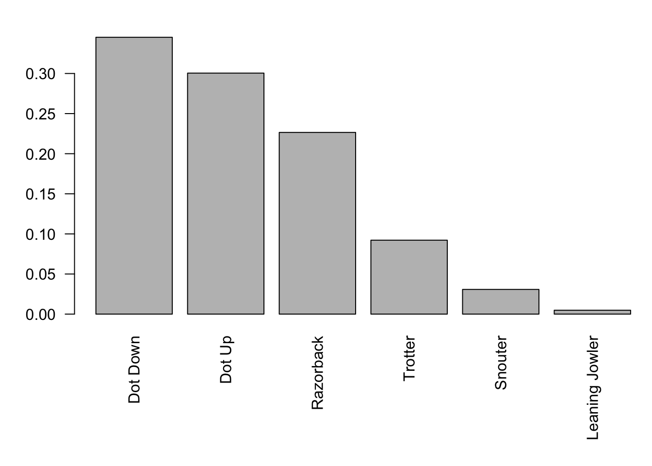

Figure 9.10: Frequency Bar Plot of Black Pig Rolls

par( mar=c(8, 4, 2, 0) )    
#The above is used to ensure that the names of the rolls are not cut off.
#The option `las = 2` is used to orient the names vertically.
barplot( sort( proportions( table( Pigs$pink ) ),
               decreasing = TRUE ), las = 2 )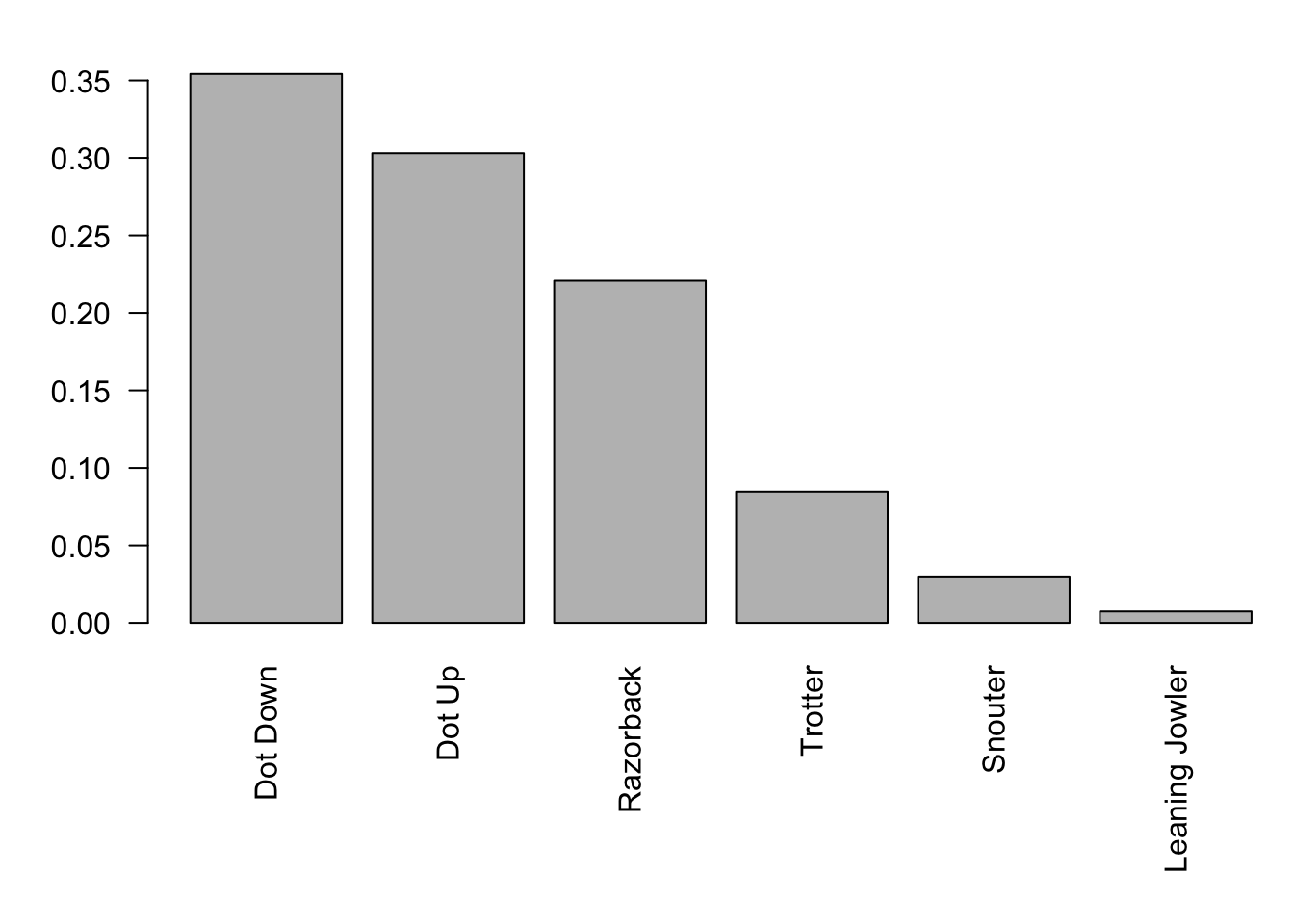

Figure 9.11: Frequency Bar Plot of Pink Pig Rolls

Based on the graphs, it appears the likelihood of each outcome is roughly the same for each pig. We can use a bit of R code to see just how close each of the outcomes were.

table(Pigs$black)[]/table(Pigs$pink)[]

## 
##       Dot Down         Dot Up Leaning Jowler      Razorback        Snouter        Trotter 
##      0.9744922      0.9917173      0.6590909      1.0257576      1.0279330      1.0889328

This says, for example, that the black pig would yield a Dot Down only approximately 97.45% as often as the pink pig would. Looking at the remainder of the values we see that the ratio that differs the most from 1 occurs for the least common outcome, the Leaning Jowler.

Example 9.25 Since our sample showed that the probability of the black pig resulting in a Leaning Jowler was less than 2/3 that of the pink pig, we have reason to at least claim that the population proportions are different. We let $p_1$ be the population proportion of the outcome Leaning Jowler for the black pig and $p_2$ be the population proportion of the outcome Leaning Jowler for the pink pig. We can thus restate our claim in terms of a formal hypothesis test.

\[\begin{align*} H_0 &: p_1 = p_2\\ H_a &: p_1 < p_2 \end{align*}\]

The function prop.test is asking us to pass to it both x as a “vector of counts of successes” and n as a “vector of counts of trials.” We can obtain the x values from the tables above and we note that both n values are 5977 as that is the length of Pigs$black or Pigs$pink.

That is, we will use x = c( 29, 44 ) and n = c( 5977, 5977 ). The only other parameter we need to set is alternative which we will set to "less" based on the structure of $H_a$ above.

prop.test( x = c( 29, 44 ), n = c( 5977, 5977 ), alternative = "less" )

## 
##  2-sample test for equality of proportions with continuity correction
## 
## data:  c(29, 44) out of c(5977, 5977)
## X-squared = 2.7014, df = 1, p-value = 0.05013
## alternative hypothesis: less
## 95 percent confidence interval:
##  -1.00000e+00  1.47924e-06
## sample estimates:
##      prop 1      prop 2 
## 0.004851932 0.007361553

As before, we will not pay attention to the two lines that offer a confidence interval.¹¹⁶ At the bottom we see the sample proportions of $\hat{p}_1$ and $\hat{p}_2$ again showing that the values do appear different at first glance. However, looking at the line which gives us our $p$-value, we see some new items. It turns out that prop.test actually uses a new distribution to find the $p$-value, the $\chi^2$-distribution.¹¹⁷ This variable (as well as its statistical counterpoint $X^2$) are explained in full detail in Chapter 11. For our purposes, we will simply focus on the $p$-value that it returns.

A $p$-value of 5.013% is higher than even our most lenient level of significance of $\alpha = 0.05$. This means that the evidence is about as extreme as it can be without being considered statistically significant. Thus, we have insufficient evidence and cannot abandon our assumption that $p_1 = p_2$ despite the disparity between $\hat{p}_1$ and $\hat{p}_2$.

Remark. Unfortunately, prop.test cannot be used to run hypothesis tests of form

\[\begin{align*} H_0 &: p_1 - p_2 = p_0\\ H_a &: p_1 - p_2 \;\Box\; p_0 \end{align*}\]

when $p_0$ is a non-zero difference. The concept of a confidence interval for $p_1 - p_2$, which we will shortly introduce in Section 9.6.4, does offer an ability to make statements about the difference between two population proportions (to some degree of confidence).

Example 9.26 In this example we will play with a new variable from the Pigs dataset, height. Looking at the dictionary for the dataset

https://statypus.org/files/PigDictionary.txt

we see that the pigs were dropped from either a height of 5 inches (height = 1) or a height of 8 inches (height = 0).

A simple question that can be asked is whether the proportion of outcomes changes based on the drop height. To do this, we will first separate our pigs into two sub-data frames as shown below. This is a bit more formulaic than the “by hand” method we used in Example 9.25

LowPigs <- Pigs[ Pigs$height == 1, ]
HighPigs <- Pigs[ Pigs$height == 0, ]

At this point, we have two different populations of values: pigs dropped from the lower height of 5 inches and pigs dropped from the larger height of 8 inches. LowPigs is a sample from the first population and HighPigs is a sample from the second populations. If we let $p_1$ be the proportion of Dot Down outcomes from the lower height and $p_2$ be the proportion of Dot Down outcomes from the higher height, we wish to run the following hypothesis test.

\[\begin{align*} H_0 &: p_1 = p_2\\ H_a &: p_1 \neq p_2 \end{align*}\]

To run prop.test, we need to pull out the number of successes for each population to create a vector. This can be done with the following code.

x1 <- sum( LowPigs$black == "Dot Down" ) 
x2 <- sum( HighPigs$black == "Dot Down" )

We also need to create a vector of counts of trials. This can be done via the following code.

n1 <- length( LowPigs$black )
n2 <- length( HighPigs$black )

We are now ready to pass our values into prop.test as vectors by using the c function which combines the values given to it into a vector.

prop.test( x = c( x1, x2 ), n = c( n1, n2 ) )

## 
##  2-sample test for equality of proportions with continuity correction
## 
## data:  c(x1, x2) out of c(n1, n2)
## X-squared = 4.5435, df = 1, p-value = 0.03304
## alternative hypothesis: two.sided
## 95 percent confidence interval:
##  -0.050980791 -0.002119533
## sample estimates:
##    prop 1    prop 2 
## 0.3318836 0.3584337

Our $p$-value of 0.03304 falls into the “gray” area between $\alpha = 0.01$ and $\alpha = 0.05$. While we do have sufficient evidence at the $\alpha = 0.05$ level of significance, the evidence is insufficient if $\alpha = 0.01.$ As such, we will leave the interpretation of this to the reader.

Remark. While you are certainly free to interpret the result of Example 9.26 as you see fit, the recommendation from Statypus would be to reserve judgment until a replication of the study could be done. Significantly smaller $p$-values may not as quickly demand replication, but anything in that “gray” area should be shown some level of doubt.

Example 9.27 We want to investigate if the proportion of children (those under the age of 18) who survived was greater than that of adults (those at least 18 years of age) who survived.

TitanicDataset <- read.csv( "https://statypus.org/files/TitanicDataset.csv" )

To begin, we can look at the first few values of the Age variable by using the head function.

head( TitanicDataset$Age )

## [1] 22 38 26 35 35 NA

We see that there are NA values in our Age variable. As we do not have the necessary values for these individuals, we will create a sub-dataframe which excludes any row where the Age variable is NA. This is done with the function !is.na¹¹⁸ which only keeps those values that are not NA.

df <- TitanicDataset[ !is.na( TitanicDataset$Age ), ]

We have chosen to simply call our new dataframe df to simplify our code and because we will quickly move on from using it directly. We can now create further sub-data frames that splits the df dataframe into two groups: children and adults.

TitanicChildren <- df[ df$Age < 18, ]
TitanicAdults <- df[ df$Age >= 18, ]

We now have data frames that represent samples of our two populations: children aboard the titanic and adults aboard the titanic. If we let $p_1$ be the proportion of children who survived and $p_2$ be the proportion of adults that survived, we wish to run the following hypothesis test.

\[\begin{align*} H_0 &: p_1 = p_2\\ H_a &: p_1 > p_2 \end{align*}\]

Now we need to extract our counts of successes as well as counts of trials. This will mimic the work we saw in Example 9.26.

x1 <- sum( TitanicChildren$Survived == 1) 
x2 <- sum( TitanicAdults$Survived == 1 ) 

n1 <- length( TitanicChildren$Survived )
n2 <- length( TitanicAdults$Survived )

Now that we have the requisite values, we can use a line of code similar to what we used in Example 9.26 except for we now include the parameter alternative = "greater".

prop.test( x = c( x1, x2 ), n = c( n1, n2 ), alternative = "greater" )

## 
##  2-sample test for equality of proportions with continuity correction
## 
## data:  c(x1, x2) out of c(n1, n2)
## X-squared = 9.2961, df = 1, p-value = 0.001148
## alternative hypothesis: greater
## 95 percent confidence interval:
##  0.06981213 1.00000000
## sample estimates:
##    prop 1    prop 2 
## 0.5398230 0.3810316

Our $p$-value of 0.001148 is very low and offers very convincing evidence that our null hypothesis, $H_0: p_1 = p_2$, should be rejected and have sufficient evidence (at any level above approximately $\alpha = 0.001$) that our claim, or alternative hypothesis of $H_a: p_1 > p_2$, is true. That is, we have very strong evidence that the proportion of all children who survived was greater than the proportion of all adults who survived.

It appears children were indeed given priority in the rescue/escape efforts!

Using techniques similar to the examples above, test the claim that the proportion of survivors who were female differed from the proportion of those who perished that were female.

9.6.3 More Than Two Samples

We initially used binom.test to run population proportion inference calculations based on one sample. We then transitioned to prop.test to run hypothesis tests coming from samples from two populations. In fact, prop.test can be used to test even more than two populations. It can be used to run tests if proportions from any number of populations are identical.

The function prop.test can be used to conduct hypothesis tests of the form

\[\begin{align*} H_0 &: p_1 = p_2 = \ldots = p_n\\ H_a &: \text{At least one of the }p_k \text{ values differs from the rest} \end{align*}\]

for $n \geq 2$ where each $p_m$ is a distinct population proportion by simply including more values in our x and n vectors.

Example 9.28 (Precision Dice) To investigate how this works, we begin by looking at data pertaining to the precision of different types of dice. The precision of dice is of utmost importance to casinos as their business is based off of knowing the probabilities in each of their games. People playing games at home also have a desire to have known probabilities and an article ¹¹⁹ on the website www.goonhammer.com did a study on different types of “precision dice.” Their data¹²⁰ can be downloaded below.

DiceRolls <- read.csv( "https://statypus.org/files/DiceRolls.csv" )

We begin by looking at the structure of DiceRolls using str.

str( DiceRolls )

## 'data.frame':    1000 obs. of  5 variables:
##  $ GW     : int  6 5 4 4 3 1 6 1 6 3 ...
##  $ NOVA   : int  3 1 3 1 3 1 5 4 5 4 ...
##  $ Baron_P: int  6 4 5 2 3 2 5 6 6 4 ...
##  $ VH     : int  4 3 5 3 3 6 6 6 2 1 ...
##  $ Casino : int  6 1 6 3 2 6 5 1 4 4 ...

This shows us that each of the five types of dice were rolled 1000 times and the result of each roll is recorded in the dataframe. We need to create a proportion from each type of dice that we can use. We will use the proportion of how often each dice rolled a 6.¹²¹

xGW <- length(DiceRolls$GW[DiceRolls$GW == 6])
xNOVA <- length(DiceRolls$NOVA[DiceRolls$NOVA == 6])
xBaron_P <- length(DiceRolls$Baron_P[DiceRolls$Baron_P == 6])
xVH <- length(DiceRolls$VH[DiceRolls$VH == 6])
xCasino <- length(DiceRolls$Casino[DiceRolls$Casino == 6])

We can combine these values into a vector which we will use as x shortly. We will also setup a diceNames vector which will allow us to label a bar plot which we will create shortly.

successes <- c( xGW, xNOVA, xBaron_P, xVH, xCasino)
diceNames <- c( "GW", "NOVA", "Baron_P", "VH", "Casino" )
successes

## [1] 142 138 175 166 167

The numbers do appear to have some variation. We should expect to see values of one sixth of a thousand or $166 \frac{2}{3}$ times, so the dice labeled VH and Casion seemed to have performed well. However, to see how different these values are, we now create a bar plot.

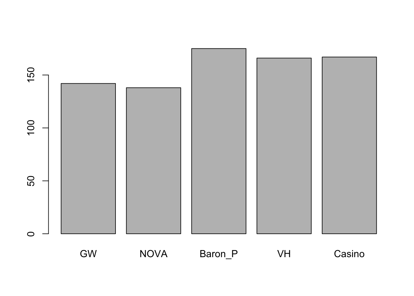
barplot( height = successes, names.arg = diceNames )

Figure 9.12: Bar Plot of 6s On Various Dice

This does give some visual evidence that the proportions of 6’s from each dice may be different. If we let $p_1$ through $p_5$ be the proportions of 6’s that each of the dice above will give ($p_1$ goes with GW, $p_2$ goes with NOVA, etc.), then we wish to run the following hypothesis test.

\[\begin{align*} H_0 &: p_1 = p_2 = p_3 = p_4 = p_5\\ H_a &: \text{At least one of the }p_k \text{ values differs from the rest} \end{align*}\]

We already have a vector of successes, called successes, so we just need to create an n vector for the number of trials. As each dice was rolled 1000 times, we can use the rep function to quickly create a vector with 5 copies of 1000.

prop.test( x = successes, 
           n = rep(1000, times = 5) )

## 
##  5-sample test for equality of proportions without continuity correction
## 
## data:  successes out of rep(1000, times = 5)
## X-squared = 8.2041, df = 4, p-value = 0.08438
## alternative hypothesis: two.sided
## sample estimates:
## prop 1 prop 2 prop 3 prop 4 prop 5 
##  0.142  0.138  0.175  0.166  0.167

This test gives us the sample estimates at the bottom showing that some of the values did stray from the theoretical expectation of one sixth. However, our $p$-value is over 8% which means that at any reasonable $\alpha$ level of significance, our evidence is insufficient to reject the assumption that the proportions of 6’s obtained from each type of dice are the same.

Example 9.29 We can restrict our view to the three most extreme dice, namely GW, NOVA, and Baron_P, and see if the outcome here is different. The code for this is below where we changed the value of times to be 3 in the rep function when defining n.

prop.test( x = c( xGW, xNOVA, xBaron_P), 
           n = rep(1000, times = 3) )

## 
##  3-sample test for equality of proportions without continuity correction
## 
## data:  c(xGW, xNOVA, xBaron_P) out of rep(1000, times = 3)
## X-squared = 6.4095, df = 2, p-value = 0.04057
## alternative hypothesis: two.sided
## sample estimates:
## prop 1 prop 2 prop 3 
##  0.142  0.138  0.175

This shows that if we were to only look at these 3 types of dice in isolation, we would have sufficient evidence, at least at the fairly relaxed $\alpha = 0.05$ level of significance, to conclude that these dice do NOT give a 6 the same proportion of the time.

In fact, we can go even further and ask prop.test to test if these three are not only equal, but all equal to one sixth.

That is, we wish to test the following:

\[\begin{align*} H_0: & p_1 = \frac{1}{6}\\ {} & p_2 = \frac{1}{6}\\ {} & p_3 = \frac{1}{6}\\ H_a: & \text{At least one of the equalities above is incorrect.} \end{align*}\]

This can be done by passing the vector p to prop.test. As shown in the New Function box for prop.test, p should be a “vector of probabilities of success. The length of p must be the same as the number of groups specified by x, and its elements must be greater than 0 and less than 1.” Since we are testing if each of these values is the same value, 1/6, we can again use the rep function to create p.

We are now able to run the hypothesis test with the following block of code.

prop.test( x = c( xGW, xNOVA, xBaron_P), 
           n = rep(1000, times = 3),
           p = rep(1/6, times = 3))

## 
##  3-sample test for given proportions without continuity correction
## 
## data:  c(xGW, xNOVA, xBaron_P) out of rep(1000, times = 3), null probabilities rep(1/6, times = 3)
## X-squared = 10.798, df = 3, p-value = 0.01287
## alternative hypothesis: two.sided
## null values:
##    prop 1    prop 2    prop 3 
## 0.1666667 0.1666667 0.1666667 
## sample estimates:
## prop 1 prop 2 prop 3 
##  0.142  0.138  0.175

This gives us even stronger evidence that at least one of the values does indeed differ from the theoretical value of $\frac{1}{6} \approx 0.167$. However, the $p$-value is still in the gray area and thus we leave the conclusion up to the reader.

9.6.4 Using `prop.test` for Confidence Intervals

As mentioned in a previous Remark, we cannot use prop.test to run hypothesis tests to see if two population proportions differ by some amount, $p_0$. However, prop.test is quite capable of computing confidence intervals of the difference of two population proportions and you have likely seen these intervals in all of the outputs from prop.test thus far. We simply need to change the parameters we pass to prop.test to ensure that we construct the confidence interval correctly, just like we did with binom.test in Section 9.5.

Example 9.30 Using the Pigs dataset which we introduced at the beginning of Section 9.6.2, we can investigate how much more likely the most likely outcome, Dot Down, is than the second most likely outcome, Dot Up. We will compute a 95% confidence interval for the difference of the two proportions and use the pink pig as our dataset. That is, if we let $p_1 =P(\text{Dot Down on Pink Pig})$ and $p_2 =P(\text{Dot Up on Pink Pig})$ be the two population proportions, we compute a 95% confidence interval for the parameter $p_1 - p_2$. This can be done with the default settings of prop.test. To use the function, we must pass both counts of successes and both total number of trials. We do this by combining the counts of successes into a vector, x, with the c() function and the same for the number of trials where the vector is now n.

prop.test( x = c( 2117, 1811 ), n = c( 5977, 5977 ) )

## 
##  2-sample test for equality of proportions with continuity correction
## 
## data:  c(2117, 1811) out of c(5977, 5977)
## X-squared = 35.273, df = 1, p-value = 2.866e-09
## alternative hypothesis: two.sided
## 95 percent confidence interval:
##  0.03421392 0.06817859
## sample estimates:
##    prop 1    prop 2 
## 0.3541911 0.3029948

This tells us that we are 95% confident that Dot Down will occur in between 3.4% and 6.8% more of all rolls than Dot Up.

If we wanted to construct an interval with more confidence, say 99%, we can alter our code as shown below.

prop.test( x = c( 2117, 1811 ), n = c( 5977, 5977 ), conf.level = 0.99 )

## 
##  2-sample test for equality of proportions with continuity correction
## 
## data:  c(2117, 1811) out of c(5977, 5977)
## X-squared = 35.273, df = 1, p-value = 2.866e-09
## alternative hypothesis: two.sided
## 99 percent confidence interval:
##  0.02893025 0.07346225
## sample estimates:
##    prop 1    prop 2 
## 0.3541911 0.3029948

Increasing our confidence to 99% requires that we extend our interval to the range between approximately 2.89% and 7.35%. This matches with our understanding of the interplay between confidence and the margin of error as well as precision.

Increasing confidence of an interval yields a higher margin of error which means that we have less precision.

Find a 90% confidence interval for the proportion of Dot Up minus the proportion of Razorback using the black pig as your sample.

Exercises

Remark. For Exercise 9.13, you will need to load the dataset BabyData1. The code for this can be found in Example 9.27.

Exercises 9.1 – 9.2 use material from Section 9.1.

Exercise 9.1 In Example 8.2 of Section 8.3, we talked about the probability that a random screw is accurate enough to be usable for a toy plane is 99%.

Treating this as $p$, what is the minimum sample size to assume the distribution of $\hat{p}$s are Normally distributed according to Theorem 9.3?
If we have samples of size $n=1000$, find $\mu_{\hat{p}}$ and $\sigma_{\hat{p}}$.
Using the values found in part b. above, find the probability that a random sample of size $n=1000$ gives a $\hat{p}$ that is less than 98%.

Exercise 9.2 Let’s revisit Exercise 8.3.

Which parts lead to sampling distributions that can be treated as being approximately Normal according to Theorem 9.3?
For all parts of Exercise 8.3 where the sampling distribution can be assumed to be approximately Normal, find $\mu_{\hat{p}}$ and $\sigma_{\hat{p}}$.
For all parts of Exercise 8.3 where the sampling distribution can be assumed to be approximately Normal, redo those parts using pnorm.

Exercises 9.3 – 9.4 use material from Section 9.2.

Exercise 9.3 Treat the 100 people in a large corporate cafeteria as a representative random sample of the entire corporation. You may assume the corporation has at least 5000 employees.

If there are 43 females in the room, give a 95% confidence interval for the proportion of female employees using the manual techniques found in Section 9.2.
If there are 43 females in the room, give a 99% confidence interval for the proportion of female employees using the manual techniques found in Section 9.2.

Exercise 9.4 Using Example 9.8 as your guide, find a 97% confidence interval for the population proportion of primary colored M&M candies if you use a sample from a party size bag and observe 610 primary colored M&M candies out of 1201 total M&M candies using the techniques of Section 9.2.

Exercises 9.5 – 9.6 use material from Section 9.3.

Exercise 9.5 You are interested in the proportion of females at the corporation is 50%, but you claim the proportion is actually lower than 50%. You observe 43 females out of 100 total people in a lunchroom. Assume we can treat this as a representative random sample of the company and that there are at least 5000 employees in the company.

What are the hypotheses you will test?
Using the techniques of Section 9.3, is there sufficient evidence at the $\alpha = 0.05$ level of significance to conclude that the proportion of females at the corporation is less than 50%?

Exercise 9.6 One of the two M&M factories in the Unites States is located in Cleveland, Tennessee. At the Tennessee factory, the proportion of primary colored M&M candies is supposed to be $p = 0.473$.¹²² You buy a party size bag and observe 610 primary colored M&M candies out of 1201 total M&M candies. Using the techniques of Section 9.3 run a hypothesis test testing if the proportion of primary colored M&M candies does not match the proportion claimed to be used at the Tennessee factory. Clearly state the hypotheses of your test and the results of it based on the choice of a significance level.

Exercises 9.7 – 9.10 use material from Section 9.5.

Exercise 9.7 Redo Exercise 9.3 using binom.test.

Exercise 9.8 Redo Exercise 9.4 using binom.test.

Exercise 9.9 Redo Exercise 9.5 using binom.test.

Exercise 9.10 Redo Exercise 9.6 using binom.test.

Exercises 9.11 – 9.14 use material from Section 9.6.

Exercise 9.11 Use prop.test and the Pigs dataset (the black pig to be precise) to see if the proportions of "Dot up" observations differs based on the height at which the pigs were dropped from. As a reminder, the dictionary for this data can be found below.

https://statypus.org/files/PigDictionary.txt

Exercise 9.12 Use prop.test and the Pigs dataset to see if the proportions of "Leaning Jowler" observations differs based on the height at which the pigs were dropped from.

Exercise 9.13 Use the TitanicDataset to determine if the proportion of female passengers differed by the passenger class of their ticket. See Example 9.28 in Section 9.6.3 for help if needed.

Exercise 9.14 Find a 97% confidence interval for the difference in population proportions of Dot Down outcomes for the pink pig based on the two different starting heights.

9.7 Appendix

9.7.1 Simulation Verification for Confidence Intervals

Example 9.31 In this example, we run a simulation to see if 95% of samples do give confidence intervals that capture $p$. We will use $p=0.6$ and $n = 50$ as we did in Section 9.2.2. We will follow the 4 Step procedure layed out in Section 6.3.2.

Step 1: Write repeatable code that performs the experiment a single time.

The code below sets up the values which will not change within each iteration of the replicate. We will run it separate and store the values in our environment to streamline our code.

n <- 50
p <- 0.6
C.Level <- 0.95    #Confidence Level
zStar <- qnorm( 1 - (1 - C.Level) / 2 )

If you want to try this code with different values, you can simply change the values above and rerun the block of code. We now use rbinom to generate a random value of successes that satisfies the now set value of $p = 0.6$ and then carry out the work done earlier in this chapter to see if the value of $p$ is in the confidence interval. It is noted that the code is slightly “slimmer” than the code we used in Section 9.2.2 to allow us to run a very large number of experiments in just a minute.

x  <- rbinom(1,n,p)                     #Random number of Successes
pHat0 = x / n                           #Sample proportion
SE = sqrt( pHat0 * (1 - pHat0) / n )    #Standard Error
MOE = zStar * SE                        #Margin of Error
#Below checks if p is in the Conf. Int.
( p > pHat0 - zStar * SE ) & ( p < pHat0 + zStar * SE )

## [1] TRUE

Step 2: Replicate the experiment a small number of times and check the results.

Now that we believe we have repeatable code, we run a small simulation (100 times should suffice) to make sure that the code is not always either TRUE or FALSE.

replicate(100, {
  x  <- rbinom(1,n,p)                   #Random number of Successes
  pHat0 = x / n                         #Sample proportion
  SE = sqrt( pHat0 * (1 - pHat0) / n )  #Standard Error
  MOE = zStar * SE                      #Margin of Error
  #Below checks if p is in the Conf. Int.
  ( p > pHat0 - zStar * SE ) & ( p < pHat0 + zStar * SE )
})

##   [1]  TRUE  TRUE  TRUE  TRUE  TRUE  TRUE  TRUE  TRUE  TRUE FALSE  TRUE  TRUE  TRUE  TRUE  TRUE  TRUE
##  [17]  TRUE  TRUE  TRUE  TRUE  TRUE FALSE  TRUE  TRUE FALSE  TRUE  TRUE  TRUE  TRUE  TRUE  TRUE  TRUE
##  [33]  TRUE  TRUE FALSE  TRUE  TRUE  TRUE  TRUE  TRUE  TRUE  TRUE  TRUE  TRUE  TRUE  TRUE  TRUE  TRUE
##  [49]  TRUE  TRUE  TRUE  TRUE  TRUE  TRUE  TRUE  TRUE  TRUE  TRUE  TRUE  TRUE  TRUE  TRUE  TRUE  TRUE
##  [65]  TRUE  TRUE  TRUE  TRUE  TRUE  TRUE  TRUE  TRUE  TRUE  TRUE  TRUE  TRUE  TRUE  TRUE  TRUE  TRUE
##  [81]  TRUE  TRUE  TRUE  TRUE  TRUE  TRUE  TRUE  TRUE  TRUE FALSE  TRUE  TRUE  TRUE  TRUE  TRUE  TRUE
##  [97]  TRUE  TRUE  TRUE  TRUE

This small simulation shows that 95 out of 100 samples generated created a confidence interval that successfully captured the population proportion. This agrees exactly with the 95% Confidence Level we set in Step 1.

Step 3: Replicate the experiment a large number of times and store the result.

We now ramp up the number of samples we test to one million to make sure that our result from Step 2 was accurate.

eventCI <- replicate(1000000, {
  x  <- rbinom(1,n,p)                   #Random number of Successes
  pHat0 = x / n                         #Sample proportion
  SE = sqrt( pHat0 * (1 - pHat0) / n )  #Standard Error
  MOE = zStar * SE                      #Margin of Error
  #Below checks if p is in the Conf. Int.
  ( p > pHat0 - zStar * SE ) & ( p < pHat0 + zStar * SE )
})

Step 4: Finally, estimate the probability using mean.

We now are able to find the proportion of the one million samples that successfully captured the population proportion which we use as the estimate of the probability that a random sample will do the same thing.

mean( eventCI )

## [1] 0.940507

This shows that only about 94% of samples result in confidence intervals that do capture the population proportion. The discrepancy between 94% and 95% is due to the inaccuracy encountered when substituting the standard error for $\sigma_{\hat{p}}$. This is a bit unsettling as what we thought was 95% Confidence is apparently only 94% Confidence.

Example 9.32 In this example, we run another simulation to see if binom.test will give better results than the manual techniques developed in Section 9.2.2. We will use $p=0.6$ and $n = 50$ as we did in Example 9.31 above.

Step 1: Write repeatable code that performs the experiment a single time.

Like before, we set up the values which will not change within each iteration of the replicate and store the values in our environment to streamline our code.

n <- 50
p <- 0.6
C.Level <- 0.95

Once again, you can simply change the values above and rerun the block of code if you want to change the parameters of the simulation. We now use rbinom to generate a random value of successes that satisfies the now set value of $p = 0.6$ and pass that result into binom.test. We first save the result as results and then look at the results.

results <- binom.test( x = rbinom(1, n, p), n = n, conf.level = C.Level )
results

## 
##  Exact binomial test
## 
## data:  rbinom(1, n, p) and n
## number of successes = 31, number of trials = 50, p-value = 0.1189
## alternative hypothesis: true probability of success is not equal to 0.5
## 95 percent confidence interval:
##  0.4717492 0.7534989
## sample estimates:
## probability of success 
##                   0.62

This sample had $\hat{p} = 0.62$ and a confidence interval of $(0.4717492, 0.7534989)$. Thus, it did capture $p$. To test this in a more repeatable way, we can use the values stored in results$conf.int.

results$conf.int

## [1] 0.4717492 0.7534989
## attr(,"conf.level")
## [1] 0.95

We can get at the individual bounds of the confidence interval using results$conf.int[1] and results$conf.int[2]. We then mimic the last line of code we used in Example 9.31 and remove all superfluous code.

results <- binom.test( rbinom(1, n, p), n, conf.level = C.Level )
( p > results$conf.int[1] ) & ( p < results$conf.int[2] )

## [1] TRUE

Step 2: Replicate the experiment a small number of times and check the results.

Now that we believe we have repeatable code, we run a small simulation (100 times is still good enough) to make sure that the code is not always either TRUE or FALSE.

replicate(100, {
  results <- binom.test( rbinom(1, n, p), n, conf.level = C.Level )
  ( p > results$conf.int[1] ) & ( p < results$conf.int[2] )
})

##   [1]  TRUE  TRUE  TRUE  TRUE  TRUE  TRUE  TRUE  TRUE  TRUE FALSE  TRUE  TRUE  TRUE  TRUE  TRUE  TRUE
##  [17]  TRUE  TRUE  TRUE  TRUE  TRUE  TRUE  TRUE  TRUE  TRUE  TRUE  TRUE  TRUE  TRUE  TRUE  TRUE  TRUE
##  [33]  TRUE  TRUE FALSE  TRUE  TRUE  TRUE  TRUE  TRUE  TRUE  TRUE  TRUE  TRUE  TRUE  TRUE  TRUE  TRUE
##  [49]  TRUE  TRUE  TRUE  TRUE  TRUE  TRUE  TRUE  TRUE  TRUE  TRUE  TRUE  TRUE  TRUE  TRUE  TRUE  TRUE
##  [65]  TRUE  TRUE  TRUE  TRUE  TRUE  TRUE  TRUE  TRUE  TRUE  TRUE  TRUE  TRUE  TRUE  TRUE  TRUE  TRUE
##  [81]  TRUE  TRUE  TRUE  TRUE  TRUE  TRUE  TRUE  TRUE  TRUE FALSE  TRUE  TRUE  TRUE  TRUE  TRUE  TRUE
##  [97]  TRUE  TRUE  TRUE  TRUE

This small simulation shows that 97 out of 100 samples generated created a confidence interval that successfully captured the population proportion. This is actually better than the 95% Confidence Level we set in Step 1.

Step 3: Replicate the experiment a large number of times and store the result.

We now ramp up the number of samples we test to one hundred thousand (one million takes a bit too long on most machines) to make sure that our result from Step 2 was accurate.

eventCIbinomtest <- replicate(100000, {
  results <- binom.test( rbinom(1, n, p), n, conf.level = C.Level )
 ( p > results$conf.int[1] ) & ( p < results$conf.int[2] )
})

Step 4: Finally, estimate the probability using mean.

We now are able to find the proportion of the one hundred thousand samples that successfully captured the population proportion which we use as the estimate of the probability that a random sample will do the same thing.

mean( eventCIbinomtest )

## [1] 0.97114

This shows that only over 97% of samples result in confidence intervals that do capture the population proportion. This means that binom.test gives confidence interval that are successful even more often the prescribed confidence level.

9.7.2 Proofs

9.7.2.1 Proof of Theorem 9.2

Proof. We use the facts that \[\mu_X = \sum_{x\in S} \big( x \cdot P(X = x)\big)\] and \[\sigma_X = \sqrt{\sum_{x\in S} \big( \left(x - \mu_X\right)^2 \cdot P(X = x)\big)}\] and make direct calculations.

\[\begin{align*} \mu_X &= \sum_{x\in S} \big( x \cdot P(X = x)\big)\\ {} &= \big( 0 \cdot P( X =0) \big) + \big( 1 \cdot P( X =1) \big)\\ {} &= \big( 0 \cdot (1-p) \big) + \big( 1 \cdot p \big)\\ {} &= p \end{align*}\]

We can now include this into the formula for $\sigma_X$.

\[\begin{align*} \sigma_X &= \sqrt{\sum_{x\in S} \big( \left(x - \mu_X\right)^2 \cdot P(X = x)\big)}\\ {} &= \sqrt{\big( (0 - p)^2 \cdot (1-p) \big) + \big( (1 - p)^2 \cdot (p) \big)}\\ {} &= \sqrt{p^2\cdot (1-p) + p \cdot (1-p)^2}\\ {} &= \sqrt{ \big( p \cdot (1-p) \big) \big( p + (1 - p)\big)}\\ {} &= \sqrt{p \cdot (1-p)}\cdot \sqrt{p + (1 - p)}\\ {} &= \sqrt{p \cdot (1-p)}\cdot \sqrt{1}\\ {} &= \sqrt{p \cdot (1-p)} \end{align*}\]

If we assumed that $N < \infty$, we could also use the definition of $\sigma$ in Section 4.2.5, but the above methods allow us prove the concept even when $N = \infty$.

See Hornsby Shire Council. for more.↩︎
To allow the use of these techniques, we need a trait that an individual has or does not have. Thus, we do not need to breakdown the different options that occur in the “Other” category here. In our situation, it contains all gender identities other than “Female.”↩︎
This is the probability that we have a proportion anywhere less than $\frac{1}{3}$ and not just the probability that the proportion is $\frac{1}{3}$.↩︎
Here, $N$ is viewed as either a large integer of $\infty$. This is part of why we don’t give an explicit formula for $p$.↩︎
Being that we let $n$ be arbitrary, we have considered all possible samples because we are allowed to use any value of $n$ that we like.↩︎
Because we our population is often so large as to make a census impossible (such as being infinite), this condition rarely comes into play and we will assume it holds for all examples in this book. If one is ever working with a population that is small enough that the sample size is more than 1% of the population size, one should invoke a “finite population correction” in their work. This concept is not shown in this book, but the interested reader can find out more by investigating https://r-survey.r-forge.r-project.org/survey/html/svydesign.html and looking at the details for the argument fpc.↩︎
If the trait we are considering is if a playing card is “red” and we are only pulling from a single deck, then even drawing a few cards can have a significant impact on the probability of the next card being “red.” This change in probability is the basis for the calculations being made by poker players. However, if we were playing with a very large number of decks, then drawing only a few cards will not significantly change the probability that the next card is red.↩︎
It is a good question as to whether we need to consider a continuity correction like the one made for the Binomial distribution. Such a correction would improve our results and, in fact, one will automatically be used when we introduce the more powerful function binom.test later in Section 9.5.↩︎
Recall that this is the situation where a stratified random sample would be ideal.↩︎
Recall that we use the value of $p$, the population proportion, and not a value of $\hat{p}$ which would come from a sample. In the future, we may have to approximate $p$ with $\hat{p}$, but when we do know $p$, we will always use that value.↩︎
This is related to the fact that $\mu_{\hat{p}} = p$.↩︎
The curious reader can look at 8.2.4 for more about information about rbinom.↩︎
Note that $2.5\% = (1 - 95\% ) / 2$ and that we could have used qnorm with lower.tail = FALSE with this value. The statypi (this stands as your official notice of the official definition of the plural form of statypus) have decided to use the value of $0.975 = 1 - (1 - 95\% ) / 2$ and not specify the value of lower.tail causing it to default to TRUE.↩︎
This approximation is literally the same one being made in the Empirical Rule, Theorem 7.3, in Section 7.6. There, we assumed that $P( -2 < z \leq 2) \approx 0.95$ which is the same thing as using the Minimum Sample Size Rule of Thumb for a $95\%$ confidence level.↩︎
In this document, we will make the simplifying assumption that a baby is born as either a boy or girl. The proportion of intersex births is a debated topic and depends heavily on the definition used for intersex. This simplification is made to make the analysis easier and is similar to assumptions such as a projectile not experiencing air resistance as it moves. Intersex births are a very real thing, but as a first pass through this topic, we will choose to simplify the world to a binary “boy/girl” choice and the interested reader is encouraged to question how the inclusion of this third gender option would affect our analysis. Someone wanting to investigate the science behind intersex births could begin with the following article by the National Library of Medicine which is run by the National Institutes of Health. https://pubmed.ncbi.nlm.nih.gov/12476264/↩︎
See this article for more information and further discussion about the difficulty in using if not just defining a $p$-value.↩︎
The practice of $p$-hacking has been found among many high level scholars in recent years. The case involving Professor Francesca Gino of Harvard University is one of the highest profile cases to date. See the LINK for an explanation of the case as of July 2024. .↩︎
There are some variations that we will investigate in Chapters 11, 13, and 14, but $H_0$ will always contain the equal sign.↩︎
We will accept the term of proving the claim at a certain level of significance. However, what it means to truly prove a claim is not fully agreed upon and should likely involve trying to replicate the results.↩︎
A version of the allegory can be found at https://www.storyarts.org/library/aesops/stories/boy.html.↩︎
It is also a song by the Platypus Baby’s favorite musician, Passenger.↩︎
The statistics community is currently generally moving away from simply taking $\alpha = 0.05$ as the default standard in nearly all cases. A lot of poorly designed experiments (and outright data fabrication) have soiled the statistics landscape and forced scholars to examine the use of $\alpha = 0.05$. Research articles have been written on the topic. See https://pmc.ncbi.nlm.nih.gov/articles/PMC6314595/ as an example.↩︎
This is the value known as double.eps in R. Using ?".Machine", we get the following information about it: “the smallest positive floating-point number $x$ such that $1 + x \neq 1$… Normally 2.220446e-16.” This is tied to how computers store numbers and related to the imprecision in floating point arithmetic.↩︎
See Wikipedia for more information.↩︎
See Wikipedia for more information↩︎
If you are curious as to this seeming discrepancy, you can begin by looking at the help file using ?binom.test.↩︎
We will look at the case of more than two populations in Section 9.6.3.↩︎
Journal of Statistics Education Volume 14, Number 3 (2006), Link.↩︎
We actually only have 5997 observations. The process of “cleaning up” the data to get to the Pigs dataframe can be found in the appendix Section 6.7.1.↩︎
While we have avoided them, the output of confidence intervals for one-tailed hypothesis tests does have valid and useful meaning. The semantics needed make the margins to give a full proof here, but basically what we are seeing is the lower 95% confidence interval as compared to the middle 95% confidence intervals we developed in Section 9.2. The lower bound of -1.00000e+00 is equal to -1 which is the lowest possible value of $p_1 - p_2$ since each $p_k$ is between 0 and 1.↩︎
The Greek letter $\chi$ is pronounced with a hard “k” sound and it rhymes with cacti or statypi.↩︎
In fact, !is.na is actually the composition of two different operators. The function is.na actually returns a logical value of TRUE if the value it sees is NA and a value of FALSE if it is anything else. The operator ! does the negation of a logical vector and thus reverses the roles of TRUE and FALSE.↩︎
See their article and GitHub for more information if you desire.↩︎
See their article and GitHub for more information if you desire.↩︎
The basic dice you used to play board games such as Monopoly or Chutes and Ladders was unlikely a precision dice. As a portion of the plastic is “removed” to create each pip, the side with only a single pip is the heaviest and thus the side opposite of 1, i.e 6, is possibly slightly favored. This is why precision dice often have their pips filled in with an equally dense material.↩︎
See this article for more information.↩︎

Chapter 9 Inference for Population Proportion(s)

New R Functions Used

9.1 Part 1: Distribution of Sample Proportions

9.1.1 Formal Setup

9.1.2 Notation

9.1.3 Set Up and Theory

9.1.4 Applications to the Distribution of Sample Proportions

9.2 Part 2: Confidence Intervals for Population Proportion

9.2.1 Confidence vs. Margin of Error vs. Precision

9.2.2 Confidence Interval Code

9.2.3 Sample Size for Desired Confidence

9.2.4 Confidence Interval Applications

9.3 Part 3: Hypothesis Test for Population Proportion

9.3.1 The Concept of a Hypothesis Test

9.3.2 The Different Types of Hypothesis Tests

9.3.3 The Code for Hypothesis Tests

9.3.4 The Boy Who Cried Wolf

9.3.5 Using an Alpha Value

9.3.6 Applications of Hypothesis Test for Population Proportion

9.4 Part 4: The Redemption of Melody

9.5 Part 5: binom.test

9.5.1 Code for binom.test

9.5.2 Applications with binom.test

9.5.3 Conditions for Inference on a Population Proportion

9.6 Part 6: Inference of Multiple Population Proportions

9.6.1 prop.test

9.6.2 Using prop.test for Hypothesis Tests

9.6.3 More Than Two Samples

9.6.4 Using prop.test for Confidence Intervals

Exercises

9.7 Appendix

9.7.1 Simulation Verification for Confidence Intervals

9.7.2 Proofs

9.7.2.1 Proof of Theorem 9.2

9.5 Part 5: `binom.test`

9.5.1 Code for `binom.test`

9.5.2 Applications with `binom.test`

9.6.1 `prop.test`

9.6.2 Using `prop.test` for Hypothesis Tests

9.6.4 Using `prop.test` for Confidence Intervals